| Issue |
Acta Acust.
Volume 10, 2026
|
|
|---|---|---|
| Article Number | 30 | |
| Number of page(s) | 16 | |
| Section | Acoustic Materials and Metamaterials | |
| DOI | https://doi.org/10.1051/aacus/2026022 | |
| Published online | 24 April 2026 | |
Scientific Article
Experimental investigation of grazing-incidence sound propagation over free-standing absorbers
Acoustics Lab, Department of Information and Communications Engineering, Aalto University, Espoo, Finland
* Corresponding author: This email address is being protected from spambots. You need JavaScript enabled to view it.
Received:
30
December
2025
Accepted:
3
March
2026
Abstract
Sound propagation at near-grazing incidence in close proximity to air-porous absorber boundaries remains an open experimental challenge. Previous investigations have reported apparent variations in sound speed near such interfaces, often based on analyses of the total sound field. In this study, sound propagation is examined using spatially resolved microphone array measurements combined with sound field separation. Two complementary analysis approaches are employed: a time-domain method based on cross-correlation-derived time-difference-of-arrival (TDOA) estimates, and a frequency-domain method relying on phase differences between selected microphone pairs to infer local propagation directions. Measurements are conducted above horizontally oriented porous absorbers of varying type and length, with corresponding free-field reference measurements. The effects of incidence angle, measurement height, and frequency are investigated. While analyses of the total sound field reproduce apparent propagation speed variations reported in earlier studies, results obtained from the isolated direct sound field indicate that the propagation speed of the directly arriving wavefront remains constant, with no evidence of physical wave bending toward the boundary. In addition, measured reflection coefficients are compared with semi-empirical predictions to further validate the experimental approach.
Key words: Porous absorbers / Bio-materials / Boundary conditions / Sound propagation / Sound field
© The Author(s), Published by EDP Sciences, 2026
 This is an Open Access article distributed under the terms of the Creative Commons Attribution License (https://creativecommons.org/licenses/by/4.0), which permits unrestricted use, distribution, and reproduction in any medium, provided the original work is properly cited.
1 Introduction
Porous absorbers are broadband sound mitigation materials widely used in architectural acoustics and noise control applications. Their effectiveness arises from a porous microstructure that allows incident sound waves to penetrate the material, where viscous and thermal interactions within interconnected pores dissipate acoustic energy [1]. Compared to resonant types such as membranes and Helmholtz resonators, porous absorbers are effective over a broader frequency range, though their performance typically diminishes at lower frequencies.
The absorption coefficient α is commonly used to quantify the energy absorbed by a surface and is defined as
 (1)
(1)
where R is the reflection coefficient. Standardized methods for measuring α include the reverberation room method for random incidence under diffuse field conditions [2], and the impedance tube method for normal incidence [3]. In addition, several in-situ and free-field techniques have been developed to estimate angle-dependent absorption coefficients and surface impedance, as reviewed in Brandão et al. [4], reflecting the need to characterize material behaviour under oblique incidence in practical applications.
While the absorption coefficient α provides a convenient measure of the energy dissipated within a material, it does not fully describe the resulting acoustic conditions near the surface. Although absorption, reflection, and surface impedance are formally linked through boundary relations, their practical manifestation governs how the sound field develops in the air region immediately above the material. Consequently, the acoustic response observed above an absorbing surface depends not only on intrinsic material properties but also on factors such as the geometry and dimensions of the absorber sample, mounting conditions, and the characteristics of the incident sound field [5]. These effects become particularly relevant under oblique and grazing incidence, where boundary interactions govern both reflection behaviour and near-surface sound propagation.
The interaction between an incident sound wave and a surface is therefore governed by acoustic boundary conditions, commonly described in terms of surface impedance. For plane-wave incidence, the surface impedance can be expressed as
 (2)
(2)
where ϕ denotes the angle of incidence. Both the surface impedance and the reflection coefficient depend on the material properties as well as on the characteristics of the incident sound field. Porous absorbers are often modelled as locally reacting surfaces for simplicity; however, due to pore interconnectivity and finite thickness, their behaviour generally exhibits extended reaction, particularly at oblique and grazing incidence [6, 7]. As a result, the effective boundary response may vary with incidence angle, frequency, wavefront shape, and material thickness.
In a homogeneous and isotropic fluid such as still air, sound propagation is characterized by a linear dispersion relation,
 (3)
(3)
where c s is the speed of sound, ω the angular frequency, and k the wave-number. This relation implies frequency-independent propagation speed under ideal conditions. Within porous media, however, sound propagation is dispersive due to viscous and thermal losses, and the effective sound speed depends on frequency through the dynamic bulk modulus and density of the medium [8]. Semi-empirical models such as the Johnson–Champoux–Allard–Lafarge model provide expressions for these quantities based on measurable material parameters [9–11].
While theoretical models generally assume an abrupt transition in propagation properties at the air-material interface, several experimental studies have reported apparent variations in sound speed in the air region immediately above porous absorbers at near-grazing incidence. Early measurements by Bedell [12] observed excess attenuation near absorbent surfaces compared to free-field predictions, suggesting wavefront distortion or a reduction in apparent sound velocity. Janowsky and Spandöck [13] subsequently investigated wavefront arrival times using vertically separated microphone pairs and reported delayed arrivals close to the surface, which they attributed to ray curvature toward the boundary. Building on this approach, more recently, Yürek et al. [14] replicated the experimental methodology using distributed array and finite-sized free-standing porous absorbers, observing frequency- and material-dependent apparent sound speed variations. More recently, distributed-array measurements and two-dimensional wavefront visualisations have reproduced and extended these near-grazing observations [15], consistent with the generalized theoretical framework proposed by Polack [16], which predicts curvature of grazing sound rays in the vicinity of finite-impedance boundaries. Building on early experimental observations by Janowsky and Spandöck and later theoretical work by Cremer and Müller [17], this formulation predicts curvature of grazing rays near finite-impedance boundaries and introduces a near-surface “adaptation layer” as a modelling construct, whose thickness is a free parameter accounting for surface admittance effects.
Accurate assessment of sound propagation in such configurations is challenging, particularly due to the coexistence of direct and scattered components and the often very limited temporal separation between their arrivals at the receiver positions. Time-difference-of-arrival (TDOA) methods based on cross-correlation between microphone signals provide a robust means of estimating propagation speed when sensor geometry, synchronization, and signal-to-noise ratio are well controlled [18]. Complementarily, frequency-domain methods based on phase differences between spatially separated sensors allow wave-number components and local propagation direction to be inferred from spatial phase gradients. Such approaches are well established in array-based sound field analysis and wavefront characterization and have been widely applied in acoustics to estimate wave-number components and local propagation properties [19–21]. When applied jointly, time- and frequency-domain analyses provide complementary insight into both the temporal and spatial characteristics of sound propagation.
Motivated by the limited availability of dedicated empirical data, this paper investigates sound wave progression at near-grazing incidence in the immediate vicinity of porous absorbing boundaries. Spatially resolved microphone array measurements in an anechoic chamber are analysed using two complementary approaches: a time-domain method based on cross-correlation-derived TDOA estimates and a frequency-domain method relying on phase differences between selected microphone pairs. Both methods are applied to direct and total sound fields, the latter enabling comparison with previous studies reporting apparent sound speed variations. The influence of material type and length along the propagation path, grazing angle of incidence (θ), and measurement distance from the boundary plane is examined.
The remainder of this paper is structured as follows. Section 2 describes the porous materials under test, the experimental setup, the sound field measurements, and the post-processing procedures. Section 3 presents the results related to the measured sound field and inferred propagation characteristics, while Section 4 discusses the findings in the context of both empirical observations and semi-empirical models.
2 Methodology
This study combines controlled anechoic measurements with time- and frequency-domain post-processing to investigate sound propagation above porous absorbers. The procedure involves impulse-response acquisition, separation of direct and indirect sound fields, frequency-dependent sound speed and wavefront analysis in time and frequency domains. Figure 1 provides a block diagram that presents the key steps.
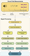 |
Figure 1. Block diagram illustrating the key stages of the methodology. |
2.1 Materials and equipment
Measurements were conducted in the anechoic chamber at Aalto Acoustics Lab. Two materials were used: glass-wool and a cellulose-based bioboard developed by Lumir. The setup included a distributed array of 16 MEMS microphones (miniDSP UMIK-X), a three-way coaxial loudspeaker (Genelec 8331A), a laser level (Bosch Professional GLL 3-50), an audio interface (MOTU UltraLite-mk3 Hybrid), and the Reaper digital audio workstation. Post-processing was performed in the MATLAB environment. The measurement setup is shown in Figure 2a, and a layout of the chamber is illustrated in Figure 2b.
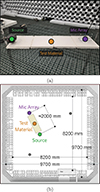 |
Figure 2. (a) Close-up image of the experimental setup. (b) Plan view of the anechoic chamber and the measurement configuration. |
2.1.1 Tested porous materials
Two types of acoustic panels, each with a surface area of 70 × 70 cm2, were used in the lining under investigation: glass wool (2 cm thick) and bioboard (3 cm thick). To ensure a uniform total thickness of 6 cm, the glass-wool panels were stacked in three layers, while the bioboard panels were arranged in two layers. Glass wool is an industry-standard porous absorber with high porosity (97%), widely used for thermal insulation and soundproofing [22]. Bioboard, developed by Lumir (Finland), is a cellulose-based acoustic panel composed of wood-derived biofibers and bio-based binders and is currently under development [23].
The acoustic tiles were positioned horizontally on the anechoic chamber’s netting without any rigid backing, corresponding to free placement in air; the supporting metal mesh was assumed to be acoustically transparent and to have a negligible influence on the material response. The length of the absorbing surface was varied by increasing the number of tiles from one to four, corresponding to a total length from 0.7 m to 2.8 m. The tiles were arranged adjacently along the propagation path. As the absorber length increased, tiles were added toward the source, while the microphone array remained fixed above the tile farthest from the source. This configuration allowed the effect of absorber length along the propagation direction to be assessed without altering the local receiver geometry.
Normal-incidence absorption of tested materials was first measured using an impedance tube to support subsequent simulations under anechoic end conditions. Four cylindrical samples (10 cm diameter) were extracted from each material and tested with rigid backing using a Brüel & Kjær Type 4206 tube. Measurements were conducted using the three-microphone method [24] across multiple sample configurations. The experimental arrangement and the tested samples are presented in Figures 3a and 3b, respectively. For completeness, the obtained normal-incidence acoustic parameters (absorption coefficient, characteristic impedance, and characteristic wave-number) are reported in the Supplementary materials (see https://acta-acustica.edp-sciences.org/10.1051/aacus/2026022/olm).
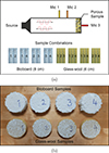 |
Figure 3. (a) Three-microphone method configuration and sample combinations. (b) Samples used for the measurements. |
The static air-flow resistivity (σ) was measured in accordance with ISO 9053 [25]. The remaining Johnson–Champoux–Allard–Lafarge (JCAL) parameters were estimated from impedance tube data using the RoKCell software (Matelys, France) [26]. These include open porosity (ϕ), high-frequency limit of the dynamic tortuosity (α∞), characteristic viscous length (Λ), characteristic thermal length (Λ′), and static thermal permeability (κ0). Parameter estimation followed the analytical approach described in Jaouen et al. [27]. Averaged parameter values are reported in Table 1.
Measured and characterised JCAL parameters.
Finally, the AlphaCell software (Matelys, France) [28] was used to simulate angle-dependent absorption coefficients under anechoic end conditions using the averaged JCAL parameter values. The results are presented in Figure 4. The simulations indicate that the largest differences between the two materials occur at shallow grazing angles (e.g., 5° or 10°) for frequencies below 800 Hz, where glass wool exhibits higher absorption. This trend reverses above 800 Hz. For grazing angles exceeding 10°, bioboard consistently exhibits higher absorption over the full frequency range.
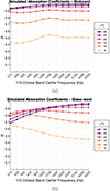 |
Figure 4. Simulated grazing-angle-specific absorption coefficients under anechoic termination conditions for (a) bioboard and (b) glass-wool. |
Additional four-microphone impedance tube measurements with an anechoic termination were carried out in accordance with ASTM E2611-24 to validate the simulation method for configurations without rigid backing [29]. Good agreement was observed between simulated and measured normal-incidence absorption coefficients.
The effective bulk modulus K(ω) and effective density ρ(ω), obtained from impedance tube measurements, were used to calculate the speed of sound inside the bioboard and glass-wool. In the bioboard, the sound speed ranges from approximately 80 m/s to 170 m/s between 315 Hz and 5 kHz, while in the glass-wool it varies from about 40 m/s to 160 m/s over the same frequency range. For both materials, the speed of sound increases with frequency.
2.1.2 Measurement setup
The microphone array comprised 16 omnidirectional MEMS microphones arranged in two rectangular grids separated vertically by 20 cm, enabling simultaneous measurements at two elevations. The array was suspended above porous samples using an adjustable microphone mount, and a counterweight minimized displacement during measurements. The source, array, and samples were aligned along a common vertical x-z plane, ensuring on-axis radiation toward the center of the absorber and symmetric receiver placement in the transverse y direction. Figures 5a and 5b show the array positioned above a single bioboard tile and multiple glass-wool tiles, respectively.
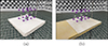 |
Figure 5. Double-grid microphone array positioned on (a) a single bioboard tile and (b) a multi-tile glass-wool configuration. Microphone positions are marked in magenta. |
Test signal was generated using a three-way coaxial loudspeaker with extended phase linearity enabled to ensure consistent delay across spectrum. The source was mounted on a custom-built, sand-filled aluminium pole (2.5 m total length) to allow elevated positioning and to cover a range of grazing incidence angles. Within the investigated range, source directivity effects were negligible. Alignment was verified using laser line projections.
In the present method, the air-material boundary is defined as the reference horizontal plane (z = 0). The grazing angle of incidence θ was then defined geometrically as the angle between the horizontal plane z = 0 and the straight line connecting the sound source to the centre of the tile farthest from the source.
2.2 Impulse response measurements
An exponential sine sweep sampled at 48 kHz and spanning 20 Hz–20 kHz was used as the excitation signal. Impulse responses were obtained by convolving the recorded sweeps with a time-reversed and amplitude-compensated version of the original signal [30]. The sound field was measured at ten receiver elevations (5–50 cm above the surface, in 5 cm steps), while the source was positioned at nine heights between 15 and 95 cm in 10 cm increments. Both the source and the array positions were adjusted manually between measurements.
For each source-array geometry, a corresponding free-field reference measurement was performed. The measurements were then repeated at the same positions for varying absorber length for both materials along the propagation path. Accounting for the dual-layer microphone array with 16 receivers, the resulting impulse response dataset has dimensions of 9 × 10 × 9 × 8, corresponding to source heights (9), receiver elevations (10), material configurations and free field (9), and receiver positions per elevation (8). In total, 6480 individual microphone signals were collected.
2.3 Signal processing and analysis
The investigation of sound propagation and potential deviations in wavefront behaviour is based on two complementary analysis approaches applied to the measured impulse responses. These include a time-domain method relying on TDOA estimates and a frequency-domain method based on phase differences between spatially separated microphone signals. Both approaches assume locally plane wave incidence at a given elevation above the porous surface and are applied consistently across the array geometry. Reference free-field measurements were analysed first to establish baseline metrics, including pressure distribution and propagation speed, against which surface-induced effects were subsequently evaluated.
Although the measurements were performed using a three-dimensional microphone arrangement, the subsequent propagation analysis was formulated in a two-dimensional (x-z) framework. This approximation is justified by the relatively small spacing between the two microphone groups in the transverse (y) direction (12.5 cm) compared to the overall source–receiver distances. As a result, transverse phase variations are expected to be negligible within the measurement region, and the sound field can be assumed locally invariant along the y-axis. Both the time-domain and frequency-domain analyses therefore focus on propagation within the vertical plane defined by the source and the surface normal.
2.3.1 Sound field separation
In an impulse response, the earliest arrival corresponds to the direct sound path, while subsequent arrivals represent reflections and secondary contributions filtered by the surface [31]. When measurements are performed close to an absorbing boundary, these secondary components can strongly bias propagation estimates if not properly isolated. Therefore, separation of the direct and indirect sound fields is a prerequisite for reliable speed and direction estimation.
The signal-subtraction approach adopted here was originally proposed by Yuzawa [32] and later refined by Mommertz [33]. The method relies on subtracting a time-aligned reference impulse response from the corresponding measurement above the surface. To achieve sub-sample temporal precision, all impulse responses were oversampled by a factor of 16 using an FIR anti-aliasing low-pass filter, enabling accurate compensation of fractional delays and amplitude discrepancies caused by arrivals occurring between sampling instants [31].
Let h 1 denote the impulse response measured above the surface and h 0 the corresponding free-field reference. The initial delay between the two responses, arising from their acquisition in separate measurement realizations with unsynchronized time origins, was estimated using cross-correlation,
 (4)
(4)
with the integer-sample delay given by
 (5)
(5)
Sub-sample accuracy was achieved using a logarithmic parabolic interpolation of the correlation peak [34], as implemented in the SDM toolbox [35],
 (6)
(6)
The total delay is then
 (7)
(7)
Temporal alignment was performed by shifting the reference response h0. Integer delays were compensated by sample-wise shifting with appropriate zero-padding, preserving the relative timing across receivers. Fractional delays were corrected using a band-limited fractional delay filter based on sinc interpolation, ensuring constant group delay across the signal bandwidth [36].
After alignment, subtraction yields the indirect sound field h 2 = h 1 − h 0, while the direct field is recovered as h 3 = h 1 − h 2. Although h 3 is mathematically equivalent to h 0, it is retained to preserve the measured arrival-time relationships across the array. All signals were subsequently downsampled to the original sampling rate.
To remove the source-receiver response and residual environmental effects, h 0 was deconvolved from h 1, h 2, and h 3. This was performed in the frequency domain by computing the auto-spectrum of the excitation S x x and the cross-spectrum S x y ,
 (8)
(8)
 (9)
(9)
where ( ⋅ )* denotes complex conjugation. To reduce spectral variance and improve numerical stability, both spectra were smoothed prior to division. A regularized transfer function was then defined as
 (10)
(10)
with the regularization parameter chosen as
 (11)
(11)
where κ is an empirically selected tuning factor. The corresponding time-domain responses were obtained by inverse Fourier transform, and the original arrival times across the array were restored by applying an inverse delay computed based on a reference receiver. Figure 6 summarizes the full post-processing chain, including delay estimation, temporal alignment, subtraction, and deconvolution.
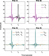 |
Figure 6. Steps of the sound field separation process: (1) determination of initial time delay (t 0 − t 1), (2) temporal alignment, (3) subtraction, (4) deconvolution. |
2.3.2 Speed estimation in the time domain
For the time-domain analysis, sound propagation delays were estimated using TDOA measurements between microphones located in different columns of the array at a given elevation. Specifically, for each elevation, the microphones belonging to the column closest to the source and the column farthest from the source were selected. This configuration maximizes the propagation distance between the sensor pair while maintaining a well-defined and repeatable geometry across all measurement configurations.
Previous studies have suggested that potential modifications of sound propagation near porous absorbers at grazing incidence may exhibit frequency-dependent behaviour [14, 16]. To investigate possible dispersion effects, the impulse responses were analysed in third-octave bands. Band-limited signals were obtained using linear-phase FIR bandpass filters of order 300, designed using the classical window method [37] and applied in zero-phase form; all processing was implemented in MATLAB using standard functions. For each frequency band, the TDOA between the selected microphone columns at a given elevation was computed using the cross-correlation-based procedure described in Section 2.3.1, yielding frequency-dependent propagation delays across the frequency range of interest.
When the geometric parameters illustrated in Figure 7 are known, the apparent sound propagation speed between the two microphone columns at a given elevation, denoted by (c′), can be calculated as
 |
Figure 7. Schematic lateral view of the measurement geometry for sound-speed estimation using the upper microphone grid. The microphone pair used in this case is highlighted in darker magenta. |
 (12)
(12)
where t denotes the measured TDOA between the selected microphone columns, and d 1 represents the difference in propagation path length from the source, given by
 (13)
(13)
with
 (14)
(14)
Here d 2 denotes the direct path from the source to the nearer microphone; d 3 the vertical distance between the source and the upper microphone grid, d 5 the horizontal distance from the source to the nearer microphone column, and d 6 the fixed horizontal spacing between the two microphone columns. When propagation speed is estimated using microphones from the lower grid, the vertical grid separation d 4 is added to d 3.
This time-domain estimate provides an apparent propagation speed along the source–receiver direction and serves as a baseline reference for interpreting trends obtained from the frequency-domain analysis presented in the following subsection, which relies on a different microphone pairing strategy.
2.3.3 Frequency-domain propagation analysis
Local propagation properties were estimated in the frequency domain using a phase-frequency fitting approach based on microphone pairs, in which time delays are obtained from a linear regression of the unwrapped cross-spectral phase as a function of angular frequency [38]. Assuming locally plane-wave and non-dispersive propagation over the analysed frequency range, TDOA between the microphones was estimated over a prescribed frequency band selected in accordance with the spatial aliasing limits imposed by the microphone spacings and practical phase robustness considerations.
The fitted TDOAs obtained from horizontally and vertically aligned microphone pairs were converted into the corresponding wave-number components. These components were subsequently used to characterize the local two-dimensional propagation direction of the sound field. The present approach is conceptually related to classical wave-number-based methods relying on spatial phase gradients, while providing improved robustness under limited spatial sampling through frequency-domain fitting.
Two-dimensional propagation parameters were evaluated at a discrete set of co-located spatial positions forming a 6 × 2 grid above the porous surface. The six vertical positions correspond to microphone elevations between 15 cm and 40 cm above the boundary, while the two horizontal positions correspond to the midpoints between microphone columns 1–3 and 2–4. These locations ensure that horizontal and vertical wave-number components describe the same local region of the sound field (see Fig. 8).
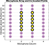 |
Figure 8. Co-located positions (indicated by yellow markers) where two-dimensional propagation parameters are evaluated using horizontal and vertical microphone pairs in the frequency-domain analysis. |
Vertical phase differences were computed using microphone pairs belonging to the same physical sub-array, which guarantees simultaneous signal acquisition and avoids uncertainties associated with sequential measurements. Consequently, the vertical spacing between paired microphones was fixed at 20 cm, corresponding to the separation between the two stacked array grids. This spacing represents a practical compromise between spatial resolution, phase robustness, and experimental repeatability.
The complex cross-spectrum between two microphone signals is defined as
 (15)
(15)
where X 1(ω) and X 2(ω) denote the Fourier transforms of the two microphone signals and ( ⋅ )* denotes complex conjugation. The corresponding phase difference is obtained as
 (16)
(16)
Assuming locally plane-wave propagation, the phase difference is related to the TDOA τ according to
 (17)
(17)
where b accounts for an arbitrary phase offset. The TDOA is estimated by performing a linear least-squares fit of the unwrapped phase difference as a function of angular frequency,
 (18)
(18)
The fitted TDOAs obtained from horizontally and vertically aligned microphone pairs are converted into wave-number components as
 (19)
(19)
where Δx and Δz denote the horizontal and vertical microphone spacings, respectively.
The local propagation angle is then obtained as
 (20)
(20)
and the magnitude of the wave-number vector,
 (21)
(21)
is reported as a complementary descriptor of the local propagation state.
3 Results
3.1 Frequency responses
The complex excess-attenuation (EA) spectra were obtained by dividing the total sound pressure by the corresponding free-field pressure, providing a frequency-dependent measure of surface-induced modifications to the sound field. Figure 9 shows the EA spectra measured 5 cm above the air-material boundary for bioboard and glass-wool at grazing angles of 4° and 23°. Results are presented for microphone column 1 (nearest to the source) and microphone column 4 (farthest from the source), and for all absorber-length configurations.
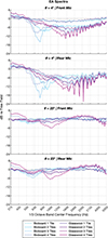 |
Figure 9. Excess-attenuation spectra measured at 5 cm above the air-material boundary for grazing angles of 4°, and 23°. |
At the shallow grazing angle of 4°, a pronounced reduction in sound pressure level is observed above approximately 500 Hz for both materials. For glass-wool, strong minima associated with destructive interference appear around 1.6 kHz when the propagation path is fully lined. In contrast, for bioboard, comparable minima occur at lower frequencies, around 700 Hz, when three tiles are present. At this grazing angle, when only a single tile is present, the sound pressure level measured at microphone column 1 remains close to the free-field reference, while a significant attenuation is observed at microphone column 4. This indicates that, for limited absorber length, indirect contributions near the source-facing side of the array are weak and primarily governed by diffraction, whereas reflections predominantly affect the downstream region.
At a grazing angle of 23°, the level differences are substantially reduced, typically remaining within ±6 dB across the measured frequency range. The dependence on absorber length becomes weaker, and the responses of the two materials converge, indicating that at steeper grazing angles the sound field is less strongly influenced by the lined surface. Across all configurations, a low-frequency amplification is observed, with its upper frequency limit increasing as the grazing angle θ increases.
Figure 10 presents the EA spectra measured at microphone column 4 for bioboard (a) and glass-wool (b), up to a height of 30 cm above the surface, at a grazing angle of θ = 4°. Results are shown for all absorber-length configurations, with the black contour indicating zero-crossings. Destructive interference effects are strongest in close proximity to the surface and gradually diminish with increasing elevation. As the absorber length increases, the low-frequency amplification becomes more pronounced and material-dependent differences become clearer. In this regime, where specular reflection is more dominant, the intrinsic material properties exert a stronger influence on the resulting sound field.
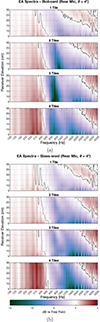 |
Figure 10. EA spectra measured at 4° grazing angle above one-to-four tiles of (a) bioboard, and (b) glass-wool tiles, as a function of microphone height (y-axis) and frequency (x-axis). Black contours indicate zero-crossing. |
Figure 11 compares the indirect field relative to the direct field for bioboard (a) and glass-wool (b), measured at microphone column 4 for a grazing angle of 4°. The lower frequency limit at which the indirect field contributes significantly shifts toward lower frequencies with increasing sample length. A finite-size effect is evident near the surface, manifested as a distinct feature around 500 Hz for both materials. In this region, the indirect field exceeds the direct field by up to 3 dB above bioboard. Measurements at larger grazing angles (not shown for brevity) indicate that glass-wool produces substantially stronger scattered sound than bioboard as θ approaches 23°, largely independent of absorber length.
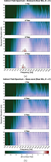 |
Figure 11. Frequency spectra of the indirect field relative to the direct field at grazing angle 4° above (a) bioboard, (b) glass-wool. Black contours indicate zero-crossing. |
It should be noted that the local grazing angle γ at the reflection point, which varies between approximately 5° and 30° depending on the receiver position, is a distinct geometric quantity from the global grazing angle of incidence θ, previously defined in Section 2.1.2. According to the manufacturer’s specifications, the loudspeaker directivity is negligible within the range of source-array geometries considered here.
3.2 Time-domain sound speed results
The time-domain analysis did not reveal any systematic frequency dependence of the estimated sound speed under either free-field or surface conditions. Accordingly, the results obtained across third-octave bands were averaged to yield a single apparent sound-speed estimate for each measurement configuration.
Figure 12 summarizes free-field sound-speed estimates as a function of microphone elevation and grazing angle. The time-domain results (Fig. 12a) provide an apparent propagation speed along the source-receiver direction. For completeness, corresponding sound-speed estimates derived from the frequency-domain analysis are also shown in Figure 12b.
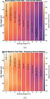 |
Figure 12. Free-field sound-speed estimates from (a) time-domain and (b) frequency-domain analyses. The primary (left) y-axis shows microphone height. Sound speed is encoded by the colour map; the colour-bar ticks are identical to those of the secondary (right) y-axis. For each grazing angle, dashed lines denote the mean sound speed and error bars indicate the range of estimates, both referenced to the secondary y-axis. |
In the time-domain results, the estimated sound speed remains within 340.4–346.6 m/s across all configurations, broadly consistent with propagation in air under the measured ambient conditions. The corresponding frequency-domain values, which are locally inferred based on microphone-pair geometry and averaged over the co-located points in microphone columns 2 and 3, fall within a slightly narrower range of 342.8–346.7 m/s and appear more closely clustered around the expected free-field sound speed.
The differences between the time- and frequency-domain sound-speed estimates arise primarily from how each method samples the source-receiver geometry and, in particular, from their shared sensitivity to the effective acoustic emission point. In the time-domain analysis, the apparent sound speed is obtained using the assumed distance between the source and each receiver, making the estimate directly dependent on the location of the emission origin. Consequently, systematic shifts in the effective source position with changing grazing angle manifest as corresponding trends in the estimated sound speed. Consistent with this interpretation, the results in both domains show an approximately linear decrease in the estimated sound speed as the grazing angle increases.
Although the frequency-domain approach does not explicitly depend on source-receiver distance, it remains sensitive to source position through array geometry. Because multiple microphone pairs at different locations are used, each pair samples a different effective acoustic emission point. As the grazing angle increases, this systematic geometric shift produces a similar near-linear decrease in the inferred sound speed. For microphone pairs located farther from the source, the local geometry increasingly approximates the global source-receiver configuration used in the time-domain analysis, causing the frequency-domain estimates to converge toward the time-domain values. For completeness, the individual free-field sound-speed estimates derived from microphone columns 2 and 3 are reported in the Supplementary materials (see https://acta-acustica.edp-sciences.org/10.1051/aacus/2026022/olm).
Figure 13 presents the relative speed of the direct sound above bioboard and glass-wool, referenced to the corresponding free-field values, for grazing angles of 4°, 9°, 17°, and 23°. Each bar represents the mean relative speed averaged over the four material configurations, while the error bars indicate the range across tile quantities.
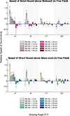 |
Figure 13. Free-field-compensated speed of direct sound above bioboard and glass-wool. Bars represent the averaged results from four material configurations. Error bars show the range across tile quantities. |
For both materials, the estimated speed remains within approximately −1 to +2 m/s relative to the free-field reference across all examined conditions. This indicates that neither absorber produces a measurable change in the propagation speed of the direct sound within the resolution of the time-domain approach. Larger deviations are observed at shallow grazing angles and at close proximity to the surface, where the interaction between the direct and surface-induced contributions is strongest. As the grazing angle increases, these deviations diminish and converge toward the free-field reference, consistent with reduced surface coupling.
3.3 Frequency-domain results
Figure 14 presents the relative deviation of the local propagation direction with respect to the free-field reference, evaluated over the frequency range 200–1200 Hz for three representative grazing angles. Results are obtained from microphone column 2 and shown as a function of microphone elevation for all material configurations. Negative values correspond to local upward bending of the propagation direction, whereas positive deviations indicate bending toward the surface. The curves were smoothed in the vertical direction using a second-order Savitzky–Golay filter.
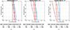 |
Figure 14. Relative deviation of the local propagation angle with respect to the free-field reference, shown as a function of microphone elevation for three representative grazing angles. Results are presented for all material configurations. Solid lines denote the total sound field, while dashed lines correspond to the isolated direct field. |
For all cases, the isolated direct field exhibits angular deviations close to zero with no systematic dependence on microphone height, confirming that the primary propagation direction remains unchanged when surface interactions are excluded. In contrast, the total sound field displays pronounced and height-dependent deviations, reflecting the influence of surface-induced scattering and interference effects. At shallow grazing angles, these deviations tend to be more pronounced at lower microphone elevations, where the interaction between the incident field and the surface is strongest. Overall, the magnitude of the deviations generally increases with the number of absorber tiles.
It should be noted that, over the range of grazing angles shown and for the analysed receiver columns (1 and 3, here) and microphone elevations, the specular reflection point never falls onto the sample when only a single tile is present. By contrast, the four-tile configuration consistently ensures that the specular point lies on the lining. For intermediate configurations with two or three tiles, whether the specular point falls onto the sample depends on both the grazing angle and the microphone elevation.
4 Discussion
Previous reports of sound wave bending and apparent sound-speed variation at grazing incidence over porous absorbers [12–15] have highlighted the importance of separating the directly arriving sound from secondary arrivals. In the present study, controlled anechoic conditions enabled the use of reference free-field impulse responses, allowing direct and indirect sound fields to be isolated through signal subtraction. This approach avoids spectral distortions associated with narrow time-windowing and provides a robust basis for propagation analysis.
Analysis of the isolated direct field using both time-domain TDOA and frequency-domain phase-gradient methods showed no evidence of sound-speed variation or wavefront bending. The estimated propagation speed and local propagation direction of the direct sound remained consistent with free-field values across frequency, elevation, and grazing angle, even at small distances from the surface. These findings indicate that the directly arriving wavefront propagates in air without measurable frequency-dependent modification under grazing incidence, and they challenge the interpretation of a frequency-dependent “adaptation layer” affecting direct sound propagation.
In contrast, analyses based on the total sound field reproduced trends similar to those reported in earlier studies, including frequency-, angle-, distance-, and material-dependent apparent variations in sound speed and propagation direction. These effects were particularly pronounced at shallow grazing angles and for longer absorbing materials, and they differed between bioboard and glass-wool, reflecting their distinct scattering and reflection characteristics.
Comparison between time- and frequency-domain results confirms that these apparent variations do not arise from changes in the propagation of the direct sound, but rather from interference between the direct and secondary components of the sound field. In this respect, the present results reconcile earlier experimental observations with classical propagation theory by demonstrating that the reported anomalies are artefacts of signal interpretation rather than true modifications of wave propagation in air.
Figure 15 compares the measured reflection coefficients with semi-empirical predictions derived from JCAL parameters. The experimental values were computed by averaging measurements from all source-receiver pairs for which the grazing angle of specular reflection fell within ±0.5° of the target value. Only measurements conducted over an absorber length of 280 cm (four tiles) were considered. Overall agreement was good, except around 500 Hz, where discrepancies emerged, and at incidence angles approaching grazing. At 500 Hz, the acoustic wavelength becomes comparable to the shorter dimension of the absorber (70 cm), enhancing diffraction and scattering effects and leading to reflection coefficients exceeding unity. These observations are consistent with the measured indirect-field spectra (see Fig. 11), which show systematically higher indirect energy around 500 Hz for bioboard than for glass-wool.
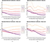 |
Figure 15. Semi-empirically predicted reflection coefficients based on JCAL parameters for (a) bioboard and (c) glass-wool. Measured reflection coefficients for (b) bioboard and (d) glass-wool. Results are averaged in 1/3 octave bands. |
The spatial distribution of interference patterns above the surface was largely governed by geometry, while their amplitude depended on material-specific reflection behaviour (see Fig. 9). This further supports the conclusion that apparent sound-speed variations observed in total-field analyses originate from the interpretation of secondary arrivals rather than from changes in the propagation of the direct wave.
The underlying cause of the illusory variations can be traced to the limited temporal separation between direct and secondary arrivals near the surface, which ranged from only a few samples to approximately fifty-nine samples (1.2 ms). When band-pass filtering is applied, this small separation leads to temporal smearing, effectively blending the direct sound with scattered components. As a result, cross-correlation or phase-based estimators yield frequency-dependent delays that do not correspond to the direct arrival alone, producing spurious variations in apparent speed and propagation direction.
Figure 16 presents time-domain impulse responses for a representative source-microphone configuration in the 315 Hz third-octave band, including both isolated direct-field (h3, 0) and total-field (h1, 0) signals. When the analysis is restricted to the direct field, the sound-speed estimate derived from the TDOA between microphone columns 1 and 4 agrees with the free-field reference within 0.2 m/s. In contrast, estimates based on the total field deviate by more than 15 m/s, owing to secondary arrivals that smear the impulse response and shift the dominant correlation peak. For this reason, and to keep the Results section focused, the corresponding total-field TDOA results are not shown. Similar interference-driven effects likely underlie earlier reports of sound wave bending at grazing incidence, including the classic experiments of Janowsky and Spandöck [13] and their modern replication by Yürek et al. [14]. Although the methodologies differ from the current one, both are susceptible to contamination from scattered and reflected components.
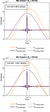 |
Figure 16. Smearing of impulse responses due to band-pass filtering: (a) front microphone (b) rear microphone. Narrow-band signal amplitudes are adjusted for visualisation. |
Although surface waves were not directly resolved in the present measurements, their potential contribution was examined analytically using measured and simulated surface impedance data. Applying established criteria for surface-wave existence provided in Attenborough [39] suggests that such waves may occur only within a limited low-frequency range and under very shallow grazing angles. However, the short source-receiver distances and limited temporal separation between arrivals in the present setup preclude unambiguous identification of surface-wave components in the time domain. Consequently, while surface waves cannot be entirely excluded as contributors to apparent anomalies observed in total-field analyses, the present results indicate that they do not affect the propagation speed or direction of the directly arriving wavefront.
The main sources of uncertainty in the present work arise from geometric tolerances and limited temperature monitoring, which may introduce small systematic variations in absolute sound-speed estimates. Finite sample size may also cause edge diffraction. Nevertheless, the use of both time- and frequency-domain analyses applied to isolated direct sound provides consistent and mutually reinforcing evidence. This convergence strongly supports the conclusion that previously reported sound-speed reductions and wave bending effects at grazing incidence are artefacts of interference, rather than manifestations of modified sound propagation in air.
5 Conclusions
Sound propagation at grazing incidence above porous absorbers was investigated using spatially resolved impulse-response measurements combined with time- and frequency-domain analyses. Across all tested configurations, including variations in absorber length, material type, and source-receiver geometry, the propagation speed of the direct wavefront remained equal to the nominal speed of sound in air. Both TDOA-based and phase-based estimates consistently showed that the directly arriving wavefront is neither slowed nor refracted, even at close distances above the surface.
In contrast, analyses based on the total sound field reproduced apparent variations in sound speed and propagation direction, similar to those reported in earlier studies. These effects were shown to arise from interference between direct and scattered components, amplified by finite absorber size, edge diffraction, and material-dependent scattering. As a result, frequency-dependent fluctuations observed in excess-attenuation spectra and apparent propagation estimates do not reflect genuine changes in propagative components.
The measured reflection coefficients showed good agreement with semi-empirical predictions based on JCAL parameters, except at very shallow grazing angles where finite-size effects become dominant. Although analytical criteria suggest that surface waves may exist within a narrow low-frequency range, their unambiguous identification was not possible under the present measurement conditions.
Overall, the results indicate that apparent near-surface propagation effects, sometimes interpreted as ray curvature, are more plausibly explained by indirect-field interference and reactive boundary contributions than by modifications of the direct sound field. These findings underscore the importance of sound-field separation when interpreting grazing-incidence measurements, particularly for in-situ and laboratory-based characterizations of finite, free-standing absorbers, and point toward the need for further investigation of such elements as used in contemporary architectural acoustics and room-acoustical treatment.
Funding
This work was funded by the Research Council of Finland’s Flagship Programme under Projects No. 318890 and 318891 (Competence Center for Materials Bioeconomy, FinnCERES).
Conflicts of interest
The authors have no conflicts to disclose.
Data availability statement
Data are available on request from the authors.
Author contribution statement
A.O.Y. conducted all measurements and analyses and wrote the majority of the manuscript. T.L. contributed to the interpretation of the results and reviewed and edited the manuscript.
Supplementary material
Table S1. Measured normal-incidence absorption coefficients of glass-wool (6 cm) and bioboard (6 cm) samples, averaged over third-octave bands.
Table S2. Complex characteristic wave numbers for glass-wool (6 cm) and bioboard (6 cm) samples, averaged over third-octave bands.
Table S3. Complex characteristic impedance for glass-wool (6 cm) and bioboard (6 cm) samples, averaged over third-octave bands.
Access Supplementary Material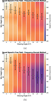 |
Figure S1. Frequency-domain free-field sound-speed estimates from (a) receiver column 2, and (b) receiver column 3. The primary (left) y-axis shows microphone height. Sound speed is encoded by the colour map; the colour-bar ticks are identical to those of the secondary (right) y-axis. For each grazing angle, dashed lines denote the mean sound speed and error bars indicate the range of estimates, both referenced to the secondary y-axis. |
References
- L. Cao, Q. Fu, Y. Si, B. Ding, J. Yu: Porous materials for sound absorption. Composites Communications 10 (2018) 25–35. [Google Scholar]
- International Organization for Standardization: ISO 354:2003 - Acoustics - Measurement of sound absorption in a reverberation room, 2003. Standard. [Google Scholar]
- International Organization for Standardization: ISO 10534-2: 2023 - Acoustics - Determination of acoustic properties in impedance tubes - Part 2: two-microphone technique for normal sound absorption coefficient and normal surface impedance, 2023. Standard. [Google Scholar]
- E. Brandão, A. Lenzi, S. Paul: A review of the in situ impedance and sound absorption measurement techniques. Acta Acustica United with Acustica 101, 3 (2015) 443–463. [Google Scholar]
- F.J. Fahy: Foundations of Engineering Acoustics. Elsevier, 2000. [Google Scholar]
- R. Dragonetti, R.A. Romano: Considerations on the sound absorption of non locally reacting porous layers. Applied Acoustics 87 (2015) 46–56. [Google Scholar]
- R. Dragonetti, R.A. Romano: Errors when assuming locally reacting boundary condition in the estimation of the surface acoustic impedance. Applied Acoustics 115 (2017) 121–130. [Google Scholar]
- Allard, N. Atalla: Propagation of Sound in Porous Media: Modelling Sound Absorbing Materials. John Wiley & Sons, 2009. [Google Scholar]
- D.L. Johnson, J. Koplik, R. Dashen: Theory of dynamic permeability and tortuosity in fluid-saturated porous media. Journal of Fluid Mechanics 176 (1987) 379–402. [Google Scholar]
- Y. Champoux, J.-F. Allard: Dynamic tortuosity and bulk modulus in air-saturated porous media. Journal of Applied Physics 70, 4 (1991) 1975–1979. [CrossRef] [Google Scholar]
- D. Lafarge, P. Lemarinier, J.F. Allard, V. Tarnow: Dynamic compressibility of air in porous structures at audible frequencies. Journal of the Acoustical Society of America 102, 4 (1997) 1995–2006. [CrossRef] [Google Scholar]
- E.H. Bedell: Some data on a room designed for free field measurements. Journal of the Acoustical Society of America 8, 2 (1936) 118–125. [Google Scholar]
- W. Janowsky, F. Spandöck: Aufbau und untersuchungend eines schallgedämpften raumes. Akustische Zeitschrift 2 (1937) 322–331. [Google Scholar]
- Yurek, J. Heldmann, T. Lokki: Bending of sound waves in the vicinity of porous materials, in: Forum Acusticum, Torino, Italy, 2023. [Google Scholar]
- Yurek, A. Öyry, T. Lokki: Two-dimensional visualisation of a travelling sound wave over porous medium, in: INTER-NOISE and NOISE-CON Congress and Conference Proceedings. Vol. 270. Institute of Noise Control Engineering, 2024, pp. 5700–5711. [Google Scholar]
- J.-D. Polack: Generalized formulation for acoustics, in: Proceedings of the 24e Congrès Français de Mécanique, Brest, France, 2019. [Google Scholar]
- L. Cremer, H.A. Müller: Die wissenschaftlichen Grundlagen der Raumakustik. Band II. S. Hirzel Verlag, Stuttgart, 1978. [Google Scholar]
- X. Li, Z.D. Deng, L.T. Rauchenstein, T.J. Carlson: Contributed review: source-localization algorithms and applications using time of arrival and time difference of arrival measurements. Review of Scientific Instruments 87, 4 (2016). [Google Scholar]
- E.G. Williams: Fourier Acoustics: Sound Radiation and Nearfield Acoustical Holography. Elsevier, 1999. [Google Scholar]
- H. Teutsch: Modal Array Signal Processing: Principles and Applications of Acoustic Wavefield Decomposition. Springer, 2007. [Google Scholar]
- J. Hald: Basic theory and properties of statistically optimized near-field acoustical holography. Journal of the Acoustical Society of America 125, 4 (2009) 2105–2120. [CrossRef] [PubMed] [Google Scholar]
- Marmoret, H. Humaish, A. Perwuelz, H. Béji, et al.: Anisotropic structure of glass wool determined by air permeability and thermal conductivity measurements. Journal of Surface Engineered Materials and Advanced Technology 6, 2 (2016) 72. [Google Scholar]
- J. Cucharero, T. Hänninen, T. Lokki: Angle-dependent absorption of sound on porous materials, in: Acoustics. Vol. 2. MDPI, 2020, pp. 753–765. [Google Scholar]
- T. Iwase, Y. Izumi, R. Kawabata: A new measuring method for sound propagation constant by using sound tube without any air spaces back of a test material, in: INTER-NOISE and NOISE-CON congress and conference proceedings. Vol. 1998. Institute of Noise Control Engineering, 1998, pp. 1265–1268. [Google Scholar]
- International Organization for Standardization: ISO 9053-1:2018 - Acoustics-determination of airflow resistance-Part 1: static airflow method, 2018. Standard. [Google Scholar]
- Matelys Research Lab: Rokcell. https://rokcell.matelys.com/. Accessed: 09.09.2024. [Google Scholar]
- Jaouen, E. Gourdon, P. Glé: Estimation of all six parameters of Johnson-Champoux-Allard-Lafarge model for acoustical porous materials from impedance tube measurements. Journal of the Acoustical Society of America 148, 4 (2020) 1998–2005. [Google Scholar]
- Matelys Research Lab. Alphacell. https://alphacell.matelys.com/. Accessed: 09.09.2024. [Google Scholar]
- ASTM International: ASTM E2611-24: standard test method for normal incidence determination of porous material acoustical properties based on the transfer matrix method, 2024. Standard. [Google Scholar]
- Farina: Simultaneous measurement of impulse response and distortion with a swept-sine technique, in: Audio Engineering Society Convention 108. Audio Engineering Society, 2000. [Google Scholar]
- P. Robinson, N. Xiang: On the subtraction method for in-situ reflection and diffusion coefficient measurements. Journal of the Acoustical Society of America 127, 3 (2010) EL99-EL104. [Google Scholar]
- Yuzawa: A method of obtaining the oblique incident sound absorption coefficient through an on-the-spot measurement. Applied Acoustics 8, 1 (1975) 27–41. [Google Scholar]
- E. Mommertz: Angle-dependent in-situ measurements of reflection coefficients using a subtraction technique. Applied Acoustics 46, 3 (1995) 251–263. [Google Scholar]
- L. Zhang, X. Wu: On cross correlation based-discrete time delay estimation, in: Proceedings of the IEEE International Conference on Acoustics, Speech, and Signal Processing (ICASSP’05). Vol. 4. 2005, pp. iv/981-iv/984. [Google Scholar]
- S. Tervo: SDM toolbox, 2018. https://se.mathworks.com/matlabcentral/fileexchange/56663-sdm-toolbox. Accessed: 09.09.2024. [Google Scholar]
- V. Valimaki, T.I. Laakso: Principles of fractional delay filters, in: Proceedings of the IEEE International Conference on Acoustics, Speech, and Signal Processing (Cat. No. 00CH37100). Vol. 6. IEEE, 2000, pp. 3870–3873. [Google Scholar]
- A.V. Oppenheim, R.W. Schafer, J.R. Buck: Discrete-Time Signal Processing, 2nd edn. Prentice Hall, Upper Saddle River, NJ, USA, 1999. [Google Scholar]
- Piersol: Time delay estimation using phase data. IEEE Transactions on Acoustics, Speech, and Signal Processing 29, 3 (1981) 471–477. [Google Scholar]
- K. Attenborough: Sound propagation in the atmosphere, in: Springer Handbook of Acoustics. Springer, 2007, pp. 113–147. [Google Scholar]
Cite this article as: Yurek A.O. & Lokki T. 2026. Experimental investigation of grazing-incidence sound propagation over free-standing absorbers. Acta Acustica, 10, 30. https://doi.org/10.1051/aacus/2026022.
All Tables
All Figures
|
Figure 1. Block diagram illustrating the key stages of the methodology. |
| In the text | |
|
Figure 2. (a) Close-up image of the experimental setup. (b) Plan view of the anechoic chamber and the measurement configuration. |
| In the text | |
|
Figure 3. (a) Three-microphone method configuration and sample combinations. (b) Samples used for the measurements. |
| In the text | |
|
Figure 4. Simulated grazing-angle-specific absorption coefficients under anechoic termination conditions for (a) bioboard and (b) glass-wool. |
| In the text | |
|
Figure 5. Double-grid microphone array positioned on (a) a single bioboard tile and (b) a multi-tile glass-wool configuration. Microphone positions are marked in magenta. |
| In the text | |
|
Figure 6. Steps of the sound field separation process: (1) determination of initial time delay (t 0 − t 1), (2) temporal alignment, (3) subtraction, (4) deconvolution. |
| In the text | |
|
Figure 7. Schematic lateral view of the measurement geometry for sound-speed estimation using the upper microphone grid. The microphone pair used in this case is highlighted in darker magenta. |
| In the text | |
|
Figure 8. Co-located positions (indicated by yellow markers) where two-dimensional propagation parameters are evaluated using horizontal and vertical microphone pairs in the frequency-domain analysis. |
| In the text | |
|
Figure 9. Excess-attenuation spectra measured at 5 cm above the air-material boundary for grazing angles of 4°, and 23°. |
| In the text | |
|
Figure 10. EA spectra measured at 4° grazing angle above one-to-four tiles of (a) bioboard, and (b) glass-wool tiles, as a function of microphone height (y-axis) and frequency (x-axis). Black contours indicate zero-crossing. |
| In the text | |
|
Figure 11. Frequency spectra of the indirect field relative to the direct field at grazing angle 4° above (a) bioboard, (b) glass-wool. Black contours indicate zero-crossing. |
| In the text | |
|
Figure 12. Free-field sound-speed estimates from (a) time-domain and (b) frequency-domain analyses. The primary (left) y-axis shows microphone height. Sound speed is encoded by the colour map; the colour-bar ticks are identical to those of the secondary (right) y-axis. For each grazing angle, dashed lines denote the mean sound speed and error bars indicate the range of estimates, both referenced to the secondary y-axis. |
| In the text | |
|
Figure 13. Free-field-compensated speed of direct sound above bioboard and glass-wool. Bars represent the averaged results from four material configurations. Error bars show the range across tile quantities. |
| In the text | |
|
Figure 14. Relative deviation of the local propagation angle with respect to the free-field reference, shown as a function of microphone elevation for three representative grazing angles. Results are presented for all material configurations. Solid lines denote the total sound field, while dashed lines correspond to the isolated direct field. |
| In the text | |
|
Figure 15. Semi-empirically predicted reflection coefficients based on JCAL parameters for (a) bioboard and (c) glass-wool. Measured reflection coefficients for (b) bioboard and (d) glass-wool. Results are averaged in 1/3 octave bands. |
| In the text | |
|
Figure 16. Smearing of impulse responses due to band-pass filtering: (a) front microphone (b) rear microphone. Narrow-band signal amplitudes are adjusted for visualisation. |
| In the text | |
|
Figure S1. Frequency-domain free-field sound-speed estimates from (a) receiver column 2, and (b) receiver column 3. The primary (left) y-axis shows microphone height. Sound speed is encoded by the colour map; the colour-bar ticks are identical to those of the secondary (right) y-axis. For each grazing angle, dashed lines denote the mean sound speed and error bars indicate the range of estimates, both referenced to the secondary y-axis. |
| In the text | |
Current usage metrics show cumulative count of Article Views (full-text article views including HTML views, PDF and ePub downloads, according to the available data) and Abstracts Views on Vision4Press platform.
Data correspond to usage on the plateform after 2015. The current usage metrics is available 48-96 hours after online publication and is updated daily on week days.
Initial download of the metrics may take a while.