| Issue |
Acta Acust.
Volume 6, 2022
|
|
|---|---|---|
| Article Number | 56 | |
| Number of page(s) | 19 | |
| Section | Noise Control | |
| DOI | https://doi.org/10.1051/aacus/2022050 | |
| Published online | 06 December 2022 | |
Technical & Applied Article
Analytical modelling and experimental validation of compliance-based low-frequency resonators for water circuits
1
Eindhoven University of Technology, 5612 AZ, Eindhoven, The Netherlands
2
ASML B.V., 5504 DR, Veldhoven, The Netherlands
* Corresponding author: This email address is being protected from spambots. You need JavaScript enabled to view it.
Received:
9
June
2022
Accepted:
10
November
2022
Abstract
Transmission losses of compact compliance-based resonators in water circuits are investigated. Experiments are performed to measure the anechoic transmission losses (TLan) of flexible-plate resonators and a gas resonator designed for frequencies between 10 and 100 Hz. The measurements are compared to theoretical results based on a lumped-element model and a finite-element model. The TLan is measured using a robust form of the multi-microphone method, which gave identical results for open and closed pipe acoustic terminations at the transmission side of the setup. When an estimate of the reflection coefficient at the termination is known, good results are obtained with only one transmission-side microphone. When TLan is high, a single microphone is sufficient on each side. For the flexible-plate resonators the TLan measurements are in agreement with theory except close to resonance, where the transmission signals are below the detection limit. Due to assumptions of a rigid cavity wall and a clamped top-plate, the theoretical resonance frequencies are too high except for the thinnest plate which displays static deformation stiffening. This deformation stiffening limits the possibility to lower the resonance frequency by using a thin flexible plate in a circuit with high static pressure. Low resonance frequencies are easier to reach with a gas resonator, in which a piston separates the water from a volume filled with air. For the gas-resonator, the measurements agree with the theoretical predictions when assuming a significant damping. The friction between the air-water-separation piston and cavity wall is suspected to cause this damping. Theory predicts that the TLan of both resonators designed for same resonance frequencies in absence of losses are equivalent. They therefore have quite similar performances except close to the resonance frequency. The flexible-plate resonator has a higher quality factor and higher (TLan) around the resonance frequency. The gas resonator is more complex and needs more maintenance but allows fine tuning of the resonance frequency by varying the gas volume.
Key words: Transmission-loss / Low-frequency / Water-circuits / Compliant-resonators / Lumped-element-model
© The Author(s), Published by EDP Sciences, 2022
 This is an Open Access article distributed under the terms of the Creative Commons Attribution License (https://creativecommons.org/licenses/by/4.0), which permits unrestricted use, distribution, and reproduction in any medium, provided the original work is properly cited.
1 Introduction
Modern day lithography machines work at nanometer precision. These machines consume power in the order of a few hundred kilowatts and dissipate a huge fraction of this power in the form of heat. Therefore the machines require cooling systems with high volumetric flow rates exceeding 0.3 m3 s−1. The cooling system generates flow noise within the fluid circuits which propagates as acoustic waves. Several measures are available to mitigate the noise at higher frequencies (f ≥ 100 Hz). However, designing a compact and efficient damper operating at low frequencies (10 Hz ≤ f ≤ 100 Hz) for high pressure (pstatic ≥ 5 bar) water circuits is not trivial. The goal of this discussion is to shed light on compact reactive dampers by means of experiments and analytical models.
There are various ways of damping or reducing acoustic pressure fluctuations which are used in aerospace, automotive, naval and civil engineering applications. Some of these use dissipative dampers which absorb acoustic energy and transform it into thermal energy. This is achieved either by use of sound absorbing materials or by providing physical resistance to dissipate acoustic power through viscous damping [1–3], like baffles and perforated tubes. At high Mach number, common in air flows, vortex shedding associated with flow separation is a very efficient dissipation mechanism [4–8]. The typical Mach numbers considered in the present application are of the order of 10−3, which implies that sound absorption by vortex shedding is not very efficient. Dissipative dampers based on porous materials work well for a large range of frequencies. However, compact dampers induce large pressure drops or are not very efficient at damping low frequency acoustic waves. Material restrictions can also prevent the use of sound absorbing materials in ultra-clean environments of the lithography machines. The second kind of dampers are reactive dampers, which reflect incoming acoustic waves in low Mach number flows. Reactive dampers usually do not increase pressure drop and can be tuned for required frequencies like for Helmholtz resonators, quarter-wave resonators, half-wave resonators and mufflers [9]. Helmholtz resonators (acoustic mass-spring systems), in which a narrow duct (neck; the acoustic mass) connects a cavity (volume; acoustic spring) to the main pipe, are the focus of our research. They can be tuned for very low resonance frequencies and theoretically have a very large transmission loss at the resonance frequency. The use of rigid Helmholtz resonators for water circuits is limited as they can get prohibitively large when designed for low frequencies (f ≤ 100 Hz) due to the low compressibility of water.
The size limitations of a rigid Helmholtz resonator can be overcome by increasing the compliance of the cavity, either by the use of a more compressible fluid in the cavity like a gas or by using a flexible plate as a cavity wall. The use of gas resonators (accumulators) is common in plumbing and naval systems to limit the transmission of sudden fluctuations in pressure [10–12]. Gas resonators can be complex with many internal components which makes them expensive. In the present case a gas resonator is considered in which a piston is used to separate the gas from the water. This allows the fine tuning of the resonance frequency by modifying the ratio of initial gas volume at atmospheric pressure to the final gas volume at the static pressure in the water flow. On the other hand, flexible-plate resonators [13–16] are simple by design, lower in cost and are virtually maintenance free. It is however more difficult to fine tune their resonance frequency. The current study focuses on experiments to compare the performance of the flexible-plate and gas resonators for resonance frequencies in the range 10 Hz ≤ f ≤ 100 Hz. Lumped-element models of the resonators are proposed, which can be used as design tools for these resonators. A single compact resonator has high transmission loss within a narrow frequency band around its resonance frequency, which can be tuned. By combining multiple compact resonators one can achieve high transmission losses in a broad frequency band [17–20].
Transmission loss measurements are typically carried out using the two-microphone method by the two-source method or the two-load method [21–24]. In principle transmission losses of a damper depend on the acoustic properties of the system on the transmission-side (as opposed to the source-side of the system). To characterise a reactive damper one prefers therefore to consider its performance when the transmission-side is an anechoic (non-reflecting) termination [22, 25]. The transmission loss under such conditions will be referred to as the anechoic transmission-loss, TLan, of the resonator. As will be shown below, there is a simple relationship between TLan and the inlet impedance Zn of the resonator. Fabricating an anechoic termination for a water circuit (without mean-flow) in the frequency range of interest is very difficult. If a pressure transducer is available in the resonator’s cavity and another one is placed at the resonator’s inlet, Zn can directly be estimated [26]. This so-called direct method cannot be used in the application considered here, because placing a microphone in the resonator cavity is not allowed in our applications. The method considered here can be used when a pressure transducer cannot be placed within the resonator. In air one often uses a multi-microphone method, which allows determining multi-port coefficients of such resonators [27, 28]. In the present case frequencies down to a few Hertz are considered, involving huge wave lengths up to 150 m. Accurate multi-microphone was not possible with the available set-up size O(1) m. In the current study a “robust” experimental procedure is developed, avoiding problems related to the inaccuracy of the multi-microphone method. Goal is to demonstrate that the measured TLan is independent of the acoustic boundary condition at the end of the transmission-side of the setup. The possibility of determining the anechoic transmission losses by means of only one microphone on each side of the resonator is also explored.
The article introduces the robust method for determining anechoic transmission loss in Section 2, based on the signals of pressure transducers placed both on the source-side and the transmission-side of the resonator. Later the article focuses on the flexible-plate resonator; namely its construction, the test setup and measurement method, the lumped-element model and experimental results in Section 3. Finally, Section 4 describes the gas resonator, the measurement method, the lumped-element model and the results. After that global conclusions are drawn.
2 Experimental method
The resonator is a volume connected to a main pipe by means of a pipe segment referred to as “neck” denoted by the index ()n (Fig. 1). There is no mean flow within the main pipe of the test-section. In a separate closed water circuit a pump forces a flow through an orifice. The pump provides low frequency noise and the flow through the orifice provides higher frequency broadband noise. This sound source is connected to the main steel pipe on which the resonator is mounted (test section) by means of a flexible polyurethane pipe. The polyurethane pipe segment reduces transmission of wall vibration from the source module to the test section. The x-axis is chosen with the origin x = 0 at the center of the junction of the neck of the resonator with the pipe. The x-axis is directed from the source side x < 0 toward the transmission side x > 0 of the setup. On each side there is an array of four microphones. The microphones on the sound-source side are denoted with the index ()A. The source-side incident and reflected plane-wave amplitudes are denoted by  and
and  . The other side of the resonator (x > 0) is connected to a duct which is in general terminated with a reflecting end, referred to as the transmission-side with index notation ()B. The transmission-side forward (transmitted) and backward (reflected) travelling plane-wave amplitudes are denoted by
  and
and  , respectively.
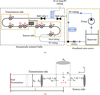 |
Figure 1 Schematic of the test-section and detailed view of the resonator neck. (a) Schematic of the experimental setup with source-side microphones (A1, A2, A3, A4) and transmission-side microphones (B1, B2, B3, B4). The entire flow system is the broadband noise source. There is no steady flow along the resonator in the main duct. (b) Schematic of the T-junction between the neck of the resonator and the main duct. The termination of the transmission side of the main pipe is either a closed end at the end of the steel tube (with closed ball-valve 1) or the PU tube termination (with closed ball-valve 2). |
At the low frequencies considered, the pressure pn at the inlet of the neck of the resonator is equal to the pressure at the inlets of the source and transmission sides of the main pipe  . This follows from Newton’s second law applied to the junction, because at the low frequencies considered the acceleration of the fluid is locally negligible. Furthermore, the mass conservation can at low frequencies be approximated as the volume flow continuity equation
  . An and Ap are the cross-sectional areas of the neck and the main pipe respectively. The flow velocity un at the resonator-neck inlet can be expressed in terms the the resonator impedance Zn un = pn. ρw is the density of water. cw,eff is the effective speed of sound in water, which was estimated by means of the Korteweg-Lamb equation [29, 30]. In the steel pipes cw,eff is very close to the speed of sound cw of pure water.Considering the particular case of an anechoic termination on the transmission-side
  of the resonator, the “anechoic” transmission loss (TLan) is calculated as [31]:
 (1)
(1)
For a finite reflection coefficient  at x = L (transmission-side termination of the setup), one can derive an expression for the ratio of incident and transmitted wave amplitudes
  in terms of RB and Zn by eliminating
  and
and  from the pressure and volume flow continuity equations. After some algebra, one finds the transmission loss with a “reflecting” termination (TLref) as:
 (2)
(2)
Note that the wave number k can be adjusted to take into account the effect of viscous damping during propagation. Assuming thin viscous boundary layers one finds [6, 32]:
 (3)
(3)
where  , dp is the inner diameter of the pipe/tube, μ is the dynamic viscosity of the fluid and ω is the angular frequency. From equations (1) and (2) the anechoic transmission loss (TLan) can be calculated for any system with a reflecting end from the measured pressure ratio
  from the following formulation (also referred as “reflection-coefficient dependent” formulation):
 (4)
(4)
Equation (4) is accurate if the reflection coefficient RB the transmission-side termination at x = L is accurately known from theory or measurements. As explained in the introduction, at the very low frequencies considered here, accurately determining RB by means of a multi-microphone method is not possible. When RB is difficult to determine, the above equation can be re-written as:
 (5)
(5)
where  is the transmitted wave amplitude for a setup with a reflecting termination. At the very low frequencies considered, the neck pressure can be approximated as the pressure measured by the microphone placed close to the neck on the transmission-side, hence,
  for frequencies satisfying the relation,
  . The index i = 1, 2, 3, … specifies the microphone considered. Here,
  is the pressure at a microphone Bi at
  .
.  is the distance between the microphone Bi and the resonator neck. The TLan estimated using equation (5) (neck pressure;
  ) with
  obtained by the multi-microphone method will be referred to as the “Multi-microphone, robust formulation”. In principle the microphone B1 closest to the neck should provide the best results. One can consider other microphones in order to obtain insight into the accuracy of the approximation. In such cases, the microphone Bi used will be specified.
Close to the resonance frequency the pressure ratio  is large and equation (5) can be approximated by:
 (6)
(6)
In this approximation the results are independent of the reflection coefficient  of the transmission-side termination. This explains why assuming
  , equation (5) is a more robust formulation than equation (4).
Three methods have been used to analyse the data. The first method is the classic multi-microphone method [33], which calculates the forward travelling wave  and the backward travelling wave
  amplitudes on the source-side (s = A) and the transmission-side (s = B) using a least-square approximation. At low frequencies (10 Hz ≤ f ≤ 100 Hz), the multi-microphone method can be inaccurate when the pressure signals at the transmission-side approach the noise floor due to high transmission loss. In particular when using equation (4), where the determination of the exact reflection coefficient RB appears to be problematic. A significant improvement in robustness of the analysis is obtained by using equation (5) assuming
  and complemented by the multi-microphone method. The reflection coefficient RB in this case need not be exactly determined.
The second method is referred to as the “source-side multi-microphone method”. This method calculates the forward travelling wave using the multi-microphone method on the source-side and calculates the transmitted wave with an estimated transmission-side reflection coefficient RB. When a reasonable estimation for RB is available the transmitted wave amplitude  can be estimated as:
![Mathematical equation: $$ {p}_B^{+}=\frac{{p}_{{B}_i}}{\mathrm{exp}\left(-\mathrm{i}k{x}_i\right)\left[1+{R}_B\mathrm{exp}\left(2\mathrm{i}{kL}\left(\frac{{x}_i}{L}-1\right)\right)\right]}, $$](/articles/aacus/full_html/2022/01/aacus220045/aacus220045-eq35.gif) (7)
(7)
where  is the amplitude of the signal of any transmission-side microphone Bi (preferably the microphone closest to the resonator, B1) at a distance xi from the resonator neck. The incident wave amplitude
  on the source-side is determined by means of the multi-microphone method. These estimations are used together with equation (5) to calculate TLan.
The third method is referred to as the “standing-wave” method. This method is based on the assumption that standing waves are dominant on the source-side of the resonator and  . Then the source-side acoustic field can be estimated with
  , hence, on the source-side one has:
 (8)
(8)
where the origin (x = 0) is at the junction of pipe and resonator neck. A single microphone on each side should then be sufficient to estimate the anechoic transmission losses (TLan). In practice the microphone A1 farthest from the junction will be used at the source-side. For the transmission-side the microphone B1 closest to the resonator will be used.
3 Flexible-plate resonator
3.1 Construction of the flexible-plate resonator
The flexible-plate resonator comprised a fluid-filled cylindrical cavity which is connected to the duct through a narrow neck by a T-junction. The diameter of the neck dn is small compared to the cavity diameter dc. The top of the cavity is covered with a circular metal plate, of uniform thickness tplate. The dimensions and the cross-sectional view of the resonator are shown in Figure 2. The resonator assembly comprised a stainless-steel base with length and height of 165 mm × 165 mm and width of 40 mm. Figure 2b shows the three-dimensional parallel perspective view of the resonator. The resonator base is shown in pink. A duct of diameter dp = 9 mm is drilled through the entire length (165 mm) of the base. The neck diameter of dn = 7.2 mm and neck length of ln = 15.5 mm is drilled through the centre of the top-face to connect with the duct. The base is connected to external ducts through attachments on the side.
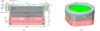 |
Figure 2 Diagram and dimensions of the flexible-plate resonator. (a) Internal dimensions of flexible-plate resonator. (b) A parallel-perspective view of the resonator. |
The top-face of the steel base mounts the aluminium cavity of the resonator (shown in grey). The cylindrical cavity with an internal diameter of dc = 150 mm is incorporated in a prismatic block of square cross section with external dimensions 165 mm× 165 mm. The height of the cavity is lc = 50 mm. The cavity has a 15 mm thick flange on the top with an outer diameter of 200 mm and inner diameter dc = 150 mm. The block and the flange are connected, they are made out of one piece (grey). The flange on the aluminium cavity is the bottom support to clamp the flexible top plate. The flange has 8 holes drilled through it at a circumference of diameter 180 mm. The cavity is fastened to the top-cover (shown in green) and the top-flange by 8 × M8 hex screws (shown in yellow) and nuts through the holes.
The cavity has a flexible plate as the top-cover (shown in green). The top-covers are circular stainless-steel plates 200 mm in diameter with 8 holes at the circumference of 180 mm to match the flange of the cavity. Five top-covers with thickness tplate = 1 mm, 2 mm, 3 mm, 4 mm or 10 mm were tested.
An aluminium top-flange (shown in blue) is used to clamp the top-cover between top flange and the flange of the cavity. Two o-rings are used within the assembly to provide a proper seal between the fastened surfaces. The fist o-ring is sandwiched between the top-cover (green) and the aluminium cavity (grey) and the second is between the aluminium cavity and the base (pink).
3.2 Test setup and measurement procedure for the flexible-plate resonator
Figure 1a shows a schematic of the setup to measure the transmission loss of the flexible-plate resonator. The setup consists of two fluid circuits. The first is the test-section, where the acoustic pressures are measured. The second fluid circuit comprised the sound source. The side of the test-section connected to the sound source is referred to as the source-side and the side of the resonator connected to the 45 m long polyurethane (PU) tube is referred to as the transmission-side.
The test-section comprised the flexible-plate resonator. The base of the resonator is coupled to stainless-steel pipes on both sides. The pipes have an inner diameter of dp = 9 mm and outer diameter of 12 mm. The pipes are coupled to the resonator an each other using SERTO® S081021-12 straight connectors. The acoustic pressures are measured using eight PCB®105C02 piezoelectric pressure transducers. The microphones were used with manufacturer’s amplitude calibration, neglecting calibration phase differences. Four microphones (transducers) are mounted on each side of the resonator at distances  and 1243.5 mm from the central axis of the resonator neck (x = 0). The microphones on the source-side are denoted as Ai and the transmission-side microphones are denoted as Bi with i = 1, 2, 3, 4. The microphones are mounted such that the normal distance between the probe surface and the pipe axis is half of pipe diameter, 4.5 mm. The stainless-steel pipes between microphones A1, A2 and microphones B3, B4 are bent in a U-shape with mean radius of curvature 38 mm. This was done in order to accommodate the entire test-section on an 1800 mm × 800 mm × 500 mm air mounted dynamic test platform by NTS®, which isolates it from transmitted ground vibration. The total length of the test-section (steel pipe) on source-side is 1.3 m and 1.49 m on the transmission-side from the resonator neck, respectively. The transmission-side of the test-section has two ball-valves. The first valve is placed at the junction between the steel pipe and a 45 m long flexible polyurethane (PU) tube with inner diameter dp = 9 mm and tube wall thickness of 1.5 mm. The second valve is placed at the end of the PU tube. When the first valve is closed it behaves as a closed-end termination with a theoretical reflection coefficient RB = 1.0 at x = L = 1.49 m. Whereas, when the first valve is open and the second valve is closed the steel pipe and PU tube junction behaves almost like an open-end termination due to the difference in the characteristic acoustic impedance of the pipes. Assuming that the PU-tube behaves as an anechoic termination the theoretical estimation of reflection coefficient RB at the PU to steel-tube junction at x = L = 1.49 m from the resonator neck is RB = −0.8 [34], which will be used in the further analysis of the transmission-loss data.
The source-side is connected to the fluid circuit with the sound source by a 1 m long PU-tube with a U-bend at a T-junction. Water is pumped through the second fluid circuit via the T-junction and through a sharp-square-edge orifice with an open-area ratio of  , where Ao is the area of the orifice opening. The orifice thickness (δo) to orifice diameter (Do) ratio is
  . The water exiting the orifice then flows into a reservoir. The orifice acts as a sound source generating a broadband acoustic wave signal which propagates towards source-side of the test-section through the PU tube. The PU-tube avoids transmission of structural vibration from the sound source to the test-section, which gives cleaner acoustic pressure measurements. The flow rate within the circuit is maintained at 91 cm3 s−1 at an absolute static pressure of 1.49 bar. The test-section is initially filled with water by opening both the valves on the transmission-side. The top-cover of the flexible-plate resonator is also kept open during the filling process to bleed out the air within the resonator cavity. Once the cavity is full, the top-cover is closed. Water is let to flow within the test-section for a minimum of 1800 s to remove trapped air bubbles. Finally, either the first or the second valve is closed to stop the flow within the test-section and begin the measurements. Once the measurements are finished the microphones are allowed to stabilise to record the electronic noise floor of the microphones. The noise signal was recorded without any water in the ducts and ensuring minimum human activity around the test setup. The PCB® pressure transducers are powered by the PCB® 483C41 eight-channel signal conditioner. The data is logged for both terminations at a sampling frequency of 4 kHz for a time-period of 500 s for all the flexible plates with an eight channel PicoScope® data logger.
3.3 Analytical model for the flexible-plate resonator impedance
In Appendix A the lumped element model for the impedance Zn of the flexible-plate resonator at the resonator neck is derived. It is assumed that the walls of the cavity, the neck and duct are rigid. The top-cover is flexible (flexible plate). Neglecting friction in the neck and inertia of the water and of the flexible plate in the cavity, the impedance (Zn) of the resonator at the neck is calculated as:
 (9)
(9)
where ω is the angular frequency, leff = 19.7 mm is the effective neck length (see Appendix A), ωc is the resonance frequency of the cavity due to the compressibility of water and ω0 is the resonance frequency of the flexible plate due to hydraulic loading. The terms ωc and ω0 are calculated as follows:
 (10)
(10)
 (11)
(11)
where dn is the neck diameter, dc is the cavity diameter, leff = 19.7 mm is the effect neck length, lc is the length of the cavity, K is the spring constant of the flexible plate (top-cover) and  is the cross-sectional area of the cavity. The spring constant K is given by [35, 36]:
 (12)
(12)
where Cr is a constant depending on the boundary conditions of the plate, E = 190 GPa is the Young’s modulus, tplate is the flexible plate thickness and ν = 0.27 the Poisson ratio of the top-cover material. For a clamped plate one has Cr = 256 and Cr ≃ 42.7 for a simply supported plate.
3.4 Influence of cavity wall flexibility
A finite-element model (FEM) was generated to verify the analytical expression (Eq. (9)) for the clamped top-cover. Finite-element model (FEM) calculations were performed using ANSYS®. The finite-element model comprised two types of elements the fluid elements (for water) and solid elements (for aluminium side-walls and the stainless steel flexible plate). The bottom surface of the aluminium cavity was given a fixed boundary condition. The steel top plate was fixed to the flange of aluminium cavity at their mating surface. Hence, the FEM takes into consideration the flexibility of the side-walls and the top plate. It is important to note here that the FEM does not include the effect of static deformation of the plate due to the static pressure in the fluid circuit. The effect of this static deformation is significant for the thinner plates. This is discussed further in Section 3.5.
Table 1 compares the calculated resonance frequencies of the flexible plate resonator from the FEM and the analytical model for a clamped top-cover. The analytical model shows good agreement with the FEM results for all top-covers with the exception of the top cover with tplate = 10 mm. The deviation between the analytical and FEM predictions is because the analytical model does not account for the elasticity of side-walls. Since the stiffness of 10 mm thick plate is greater compared to the stiffness of the aluminium cavity, the stiffness of the cavity defines the natural frequency of the resonator, which is not predicted by the analytical model. For the thicker plates the perfect clamping of the plate assumed by the FEM model is not realistic. The behaviour actually approaches that of a simply supported plate. A lumped element for a simply supported plate and rigid cavity side walls is therefore considered for comparison.
Comparison of resonance frequencies of the flexible-plate resonator with different plate thicknesses using analytical model, finite-element model (FEM) and experiments.
3.5 Results of transmission loss measurements
Figure 3 shows the comparison between power spectrum density (PSD) plots of acoustic pressures at the source-side and transmission-side microphones for the flexible-plate resonator with tplate = 2 mm. Figure 3a plots the PSD for the setup terminating with a 45 m polyurethane tube (with RB ≃ −0.8). Figure 3b plots the PSD for the setup terminating with the closed-end (RB = 1). In both cases RB is the reflection coefficient at x = L = 1.49 m. The PSD curves were plotted using a moving average of 5 data points over the entire frequency range to reduce the scatter. At f > 5 Hz the pressure amplitudes measured by the source-side microphones (A1 through A4) decrease linearly as a function of the microphone distance (xi) from the resonator neck, for both terminations. This indicates a standing wave on the source-side for f > 5 Hz. The source-side pressures are generally above the noise-level between the 1 Hz and 200 Hz for both terminations. As the signal-to-noise ratio of the source-side microphones is high for the relevant frequency range, both the standing wave method and the multi-microphone method can be applied. Please note, the sharp peaks in the amplitude that are observed at 50 Hz, 150 Hz and 250 Hz. The peaks are a result of the 50 Hz grid frequency.
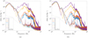 |
Figure 3 Power spectrum density plots of acoustic pressures measured at source-side (solid lines) and transmission-side microphones (dashed lines) of flexible-plate resonator with tplate = 2 mm for (a) the 45 m PU tube termination and (b) the closed-end termination on the transmission-side. At the resonance frequency of 37 Hz, the transmitted signal is close to the noise floor. |
For frequencies f < 5 Hz, the PSD of transmission-side pressures reach values close to that of the source-side pressures, indicating that the resonator is less effective. It is important to note that below f = 5 Hz one sees from Figure 3 that the signal is independent of the microphone position and is almost the same for the source and transmission sides. One therefore expects that the transmission loss data is meaningless at these low frequencies. Close to resonance frequency the pressure amplitudes approach the noise floor. Indeed, one expects the pressure at the inlet of the resonator neck to vanish at resonance (as pn ≃ 0). The pressure amplitudes on the transmission-side are dependent on the type of termination at x = 1.49 m. Above f > 300 Hz one also observes that the PSD plots (in Fig. 3) of the pressure signals on the source-side and the transmission-side approach the noise floor. Therefore the measured TLan at frequencies f > 300 Hz can be disregarded. Therefore the relevant frequency range for the transmission-loss measurements is between 5 Hz ≤ f ≤ 300 Hz.
Figures 4a and 4b compare the three methods of calculating TLan from experiments for both terminations discussed in Section 2. It should be noted that the measured TLan values were smoothed using a moving average over the entire frequency range with 5 data points. The classic multi-microphone method is compared for both terminations using the robust formulation ans the reflection-coefficient dependent formulation. The source-side multi-microphone method is denoted by “Source-side MM/Bi”, where Bi denotes the transmission-side pressure transducer. The TLan is also calculated using the standing-wave method. The source-side multi-microphone method and the classic multi-microphone method using the robust formulation agree well with each other for almost the complete frequency range (5 Hz ≤ f ≤ 300 Hz) irrespective of the microphone used to estimate the transmission-side travelling wave with typical average deviations less than 2 dB. The standing wave method agrees with the former two methods close to the resonance frequency and starts deviating at low-frequencies. Since the standing wave method utilises only two microphones (one on each side), it is a relatively simple method to achieve a rough estimate of the transmission loss of the resonator. It should also be noted that in case of the closed-end termination (in Fig. 4), the source-side multi-microphone method shows a peak close to f ≃ 238 Hz. This frequency corresponds to the quarter wave frequency between the resonator neck and the closed-end. This proves the robustness of equation (5). The drawback of the reflection-coefficient dependent-formulation (Eq. (4)) in comparison to the robust-formulation (Eq. (5)) of TLan is apparent in Figure 4b as it shows a deviation of 10 dB for the closed-end boundary condition. Equation (4) is strongly dependent on accurate measurement of reflection coefficient of the termination. The robust-formulation on the other hand is weakly dependent on the reflection coefficient, which greatly reduces the uncertainty in TLan calculation (in the Fig. 4c). Hence, one does not need an accurate estimation of reflection-coefficient of the termination.
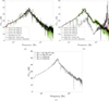 |
Figure 4 Comparison of measured TLan calculated using source-side multi-microphone, classic multi-microphone method with robust and reflection-coefficient dependent formulation, and the standing-wave method for flexible-plate resonator with tplate = 2 mm for (a) the 45 m PU-tube (RB = −0.8) termination, and (b) the closed-end termination (RB = 1) on the transmission-side. The effect of error in the estimated reflection coefficient RB on measured TLan is shown in (c). |
Figure 4c demonstrates the effect of errors in the estimated RB on the measured TLan. The TLan was calculated using the correct estimation of reflection coefficient (RB = −0.8) for the 45 m long PU tube and compared to the TLan with a wrong estimation of RB = 0. Similarly TLan was also calculated for closed-end termination with RB = 1 and compared to TLan with wrong estimation of RB = 0. Even with a drastic error of 100% in the estimated RB of the end transmission-side the measured TLan deviates less than 2 dB. This is because the acoustic pressure ratio, between source and transmission-sides, is very large,  . Hence, the result is globally independent of the estimated value of RB as long as the transmission-side pipe segment is not resonant. However some local deviations are observed in TLan, which are suspected to be due to transmission of vibration through pipe-walls.
The effect of structural vibration on the measured TLan is shown in Figure 5. The anechoic transmission losses TLan of the flexible-plate resonators with tplate = 1 mm and 2 mm are measured with two configurations. Firstly, the test-section was rigidly connected to the sound-source section using steel-tubes of 9.0 mm internal diameter. Secondly, the setup was dynamically isolated from the sound source by a 1 m long PU tube with a U-bend. The bent PU-tube reduces the propagation of structural vibration, while allowing acoustic wave transmission through the fluid. Figure 5 shows that dynamic isolation of the measurement section from the sound source has a significant effect on the measured TLan at frequencies close to and above resonance frequency. When setup is rigidly linked to the sound-source the measured TLan shows a more complex behaviour and lower TLan at some frequencies due to transmission of vibrations through structure. The TLan measured by the isolated system shows an expected behaviour. The transmission through wall vibration has also been reported by Liu and Yang [11] in a study of liquid–gas filled Helmholtz-resonator arrays for sea-water piping systems.
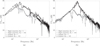 |
Figure 5 Comparison between measured TLan of a dynamically isolated test setup and a rigidly connected test setup to the sound source (orifice). The TLan was calculated using the multi-microphone method for flexible plate resonator with tplate = 1 mm (a) and 2 mm (b). |
Note that even with isolation of the test section from the sound-source and pump section by means of a 1 m long poly-urethane pipe section does not completely isolate the test-section from wall vibrations.Around the resonance frequency (maximum transmission loss) the TLan curve for the tplate = 1 mm thick plate deviates strongly from the shape expected for a simple resonator (Fig. 5). There are wiggles, weaker but similar to those observed when the signal is polluted by wall vibration. The curve for the tplate = 2 mm has a shape closer to the expected shape with a single sharp peak. As already discussed previously that the measurements close to the resonance frequency are not reliable for the flexible-plate resonators. A consequence of this, is that one cannot evaluate the quality factor of these resonators. From the measurements of TLan for the tplate = 2 mm resonator, one concludes that the quality factor of the resonator is  , with f0 = 37 Hz the resonance frequency and Δf3dB ≃ 10 Hz the resonance peak width at 3 dB below the maximum of TLan. This is much higher than the value estimated for the gas resonators.
Also a point to note here is the effect of change in speed of sound on the resonance frequency between a water-filled elastic duct and a water-filled rigid duct. For a thin flexible plate (tplate < 4 mm), the cavity impedance is dominated by the stiffness of the flexible plate. The compressibility of water comes into effect when the ratio of resonance frequencies  in equation (9) is
  . Since in a steel duct the effective speed of sound cw,eff is 4% lower than cw, the ratio
  . Hence, in most practical cases the effect of change in speed of sound in a steel pipe relative to that of bulk water can be neglected.
Figure 6 shows the comparison between measured, analytical model and finite-element-model (FEM) calculations of TLan. The measured TLan are calculated using the classic multi-microphone method for termination with 45 m PU-tube (RB = −0.8) and the closed-end termination (RB = 1). The TLan plots have been smoothed using the moving average with 5 data points over entire frequency range. The measured resonance frequencies for the 1 mm flexible plate is higher than the frequency predicted by the analytical model with clamped plate. The study by Plaut [37] shows an increase in stiffness is due to the non-linear deformation of thin plates. This deformation is determined by the dimensionless parameter  . For a static pressure difference across the plate of Δp = 49 kPa, Young’s module of
  GPa, plate diameter dc = 150 mm and plate thickness tplate = 1 mm one finds the value
  . From the results by Plaut [37] a 43% increase in stiffness is found. This corresponds to a 20% increase in the resonance frequency of the flexible plate resonator. From the experiments a deviation of 11% was measured at a static pressure of 49 kPa. This lower effect of non-linear static deformation on the frequency than the theoretical prediction of Plaut [37] is expected to be due to the flexibility of the aluminium cavity. It is important to note that this effect depends on
  .
.
 |
Figure 6 Comparison between measured, analytically estimated and FEM estimated TLan of flexible plate resonators with tplate = 1 mm (a), 2 mm (b), 3 mm (c), 4 mm (d) and 10 mm (e). The measured TLan have been calculated using the multi-microphone method for both terminations. The adjusted frequency fit TLan value is estimated from a visually guess of the maximum response frequency fmax from the measurements. |
Hence the static deformation is reduced by a factor 16 for tplate = 2 mm compared to tplate = 1 mm, it is negligible for thicker plates. The increased plate rigidity due to non-linear deformation limits the use of thinner or wider plates when aiming at a very low resonance frequency. Of course high static pressures precludes the use of very thin plates because of possible rupture. This makes the use of the more complex gas resonators interesting as alternative to flexible plate resonators.
The resonance frequencies of the resonator with tplate = 2 mm, 3 mm and 4 mm fall between the clamped and simply-supported analytical models. The measured resonance frequencies approach the simply-supported case as the plate thickness increases. This is because the clamping of steel top plate onto the cavity with aluminium flanges does not behave like a fixed plate, rather it has a behaviour in between the fixed and the simply-supported plate. As the top plate gets thicker, the clamping behaves more closer to a simply-supported plate, which reduces the resonance frequency of the resonator. The measured TLan plots are fitted to theoretical TLan plots with maximum response frequencies (fmax) that are visually adjusted to the experimental results. These plots predict within 2 dB the TLan over a wide frequency range  and
and  .
.
It is observed that the resonance frequency of 10 mm thick flexible plate is found to be lower than the simply-supported analytical model because the analytical model assumes rigid cavity walls. In the case of tplate = 10 mm the stiffness of the plate and the cavity wall is comparable, hence the compliance of the aluminium wall of the cavity also determines the resonance frequency. The FEM prediction considers the side wall compliance, but assumes a perfectly clamped plate. The effects of the side wall compliance and failure of the clamping are of the same order of magnitude for the thickest plate. The failure of the clamping for thicker plates is difficult to describe in a FEM model. An accurate model should actually predict the finite non-uniform separation of the plate from the ring and side wall as a result of the static pressure and the complex three dimensional deformation due to the fixing bolts. Table 1 compares the resonance frequencies of the flexible-plate resonator for all the cases.
The maximum observed transmission loss for the flexible-plate resonator is limited to 50 dB for tplate = 1 mm and 2 mm and 30 dB for tplate = 10 mm. When effect of friction due to fluid viscosity and inertia of water are considered the resonator can still achieve a maximum theoretical anechoic transmission loss of 80 dB (see Appendix A), which cannot explain the deviation.
The maximum theoretical anechoic transmission loss (TLan) of the flexible-plate resonator (close to resonance frequency) is proportional to the logarithm of  . This is seen from equation (1). Hence, to increase the TLan of the resonator one has to reduce the effective neck length leff of the flexible-plate resonator by reducing the dimension of the neck length. However, reducing the leff alone would alter the resonance frequency. Therefore, one also has to reduce the neck diameter to keep ratio
  the same, thereby maintaining the same resonance frequency (ω0). The main advantage of flexible plate resonators is that they are cheap and are almost maintenance free. One can therefore easily use them in arrays tuned for optimal reduction of transmission. A compact resonator for very low frequencies however involves a thin plate which can be problematic when high static pressures are used in the water circuit. The gas resonator is a more complex resonator, which however is easier to design for higher static pressure applications.
4 Gas resonator
4.1 Construction of the gas resonator
Figure 7 shows the schematic of construction of the gas resonator used in the experiments. The gas resonator assembly comprises a cavity, a free-floating piston and a bellow. The resonator cavity has an inner diameter of dc = 150 mm and outer diameter of 160 mm and a height of 172 mm. The cavity is made of stainless-steel. The cavity of the resonator is divided into two sub-cavitys namely the gas-cavity and the water-cavity by the free-floating piston. The piston is attached to the resonator cavity by means of a bellow. The piston has the same diameter as the resonator cavity dc. The piston maintains a pressure equilibrium between the water and the gas. The piston is made of stainless-steel with a PTFE seal ring at its circumference. The bellow in conjunction with the piston prevent leakage of gas into the water-cavity. The gas-cavity filled with a known volume of pressurised gas provides the compliance of the resonator. The gas-cavity has a pressure valve on the top, which is used to fill it with a user-specified gas-pressure. The water-cavity is filled with water from the fluid-circuit by a narrow-neck. The resonator neck has a diameter dn = 10.26 mm with a length ln = 1.22 mm, the narrow neck expands into a wider duct with diameter dN = 23 mm and length lN = 35 mm. The wider duct connects to the water-cavity.
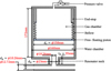 |
Figure 7 Cross-sectional view of of the gas resonator. Gas in the gas-cavity is separated from the water in the water-cavity by a free moving piston attached to a bellow. |
The neck connects to the fluid duct by a T-junction. The fluid filled steel ducts in the circuit have an inner diameter of dp = 10.26 mm and outer diameter 12.72 mm. The resonator duct is connected to external ducts using 12.7 mm Swagelok® straight connectors. All the parts are made out of stainless-steel.
The upward motion of piston is restricted by an end-stop within the gas-cavity. The maximum gas volume when the piston is at the bottom-end of the cavity is 2.00 dm3. When piston is at the top-end of the cylinder, the gas volume is 0.80 dm3. Hence, the gas-cavity has an operational volumetric range of 1.20 dm3.
4.2 Test setup and measurement procedure for the gas resonator
The layout of the experimental setup to test the gas resonator closely resembles the schematic in Figure 1a, however there are some differences. The gas resonator is connected to stainless-steel tubes with dp = 10.26 mm and 12.7 mm outer diameter. Three PCB®105C02 piezoelectric dynamic pressure transducers are mounted on each side of the test-setup at distance of 130 mm, 480 mm and 1439 mm from the central axis of the resonator neck. These are denoted as microphones Ai on the source-side and Bi on the transmission-side with i = 1, 2, 3. The stainless-steel tubes connecting the microphones A1 and A2 on the source-side, and the microphones B2 and B3 are bent in a U-shape with a mean radius of curvature of 51 mm. The bent pipes help accommodating the entire measuring section onto the THORLABS® NEXUS 2 m × 1.2 m × 0.31 m anti-vibration table. The total length of the steel tubes connected to the gas resonator on each side is 1.6 m from the central axis of the resonator neck. The steel tubes and the pressure transducer mounts were coupled using 12.75 mm Swagelok® straight connectors. The transmission-side of the test-section is connected a 20 m polyurethane (PU) tube with a ball-valve. The other end of the PU tube is terminated with a second ball-valve. The PU tube has an inner diameter dp = 10.26 mm and outer diameter of 12.7 mm. The closing of the first ball-valve is equivalent to a closed-end termination with reflection coefficient RB = 1. When the first ball-valve is open and the second ball-valve is closed, the transmission-side of test section terminates with the 20 dB PU tube with reflection coefficient RB ≃ −0.8.
The end of the steel tube on the source-side of the test section is connected to one end of a T-junction consisting of the noise source with a 1 m long PU tube. The PU tube avoids transmission of structural vibration from the source to the test-section. The second end of the T-junction is connected to the supply line of the pump with a 5 m long polyurethane tube. The third end is connected to the orifice, which is connected to the return line of the pump. The orifice is made of stainless-steel with an open-area ratio of  . The orifice is within a stainless-steel pipe of internal diameter 7.5 mm. The orifice hole diameter Do is 3.5 mm and the thickness (δo) to the hole diameter (Do) ratio is
  . The pump circulates the water through the flow circuit (and the orifice) at 1.8 × 10⁻⁴ m3 s−1. The orifice combined with the pump generates a broad-band noise signal, which propagates towards the test-section. The pressures were measured twice for a time period of 1200 s using the PAK® MKII is a high-speed multi-channel data acquisition system at a sampling frequency of 12 kHz.
Figure 8 shows the operation procedure of the gas resonator. Initially the water in the fluid circuit is drained and the gas-cavity of the resonator is filled through the valve on the top. Once the gas pressure within the gas-cavity reaches a stable initial absolute gas pressure p0 the pressure valve is closed. The pressures were measured using Comark® C9557 differential manometer to a precision of 1 mbar. An uncertainty of 20 mbar is present due to fluctuations in atmospheric pressure patm, which was not monitored. Due to the absence of static pressure within the fluid circuit and higher gas pressure (p0 − patm) in the gas-cavity the piston the piston reaches the bottom stop of the resonator cavity, extending the cavity to the maximum volume. Hence, the initial volume of the cavity is V0 = 2.00 dm3.
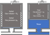 |
Figure 8 Operation procedure of the gas resonator. The gas-cavity is is initially filled with air at absolute pressure p0 by using a gas inlet valve on top of the resonator without any static pressure from fluid circuit, hence gas-cavity has initial volume V0. Once the pressure in the water circuit is increased up to the final pressure pf the volume of the gas-cavity reduces from V0 to Vf. |
After filling the gas, the fluid circuit is pressurised with water to a static pressure pf. The fluid exerts a back-pressure on the gas cavity compressing it. The gas cavity reduces in volume and reaches a final stable absolute pressure pf which is measured in the similar way as p0. Assuming isothermal compression of the gas-cavity the final gas volume Vf is calculated as:
 (13)
(13)
Once the final pressure pf and volume Vf of the gas-cavity are known, the acoustic pressure data are recorded by the microphones. The gas resonator was tested for four initial gas pressures p0 = 2.60 bar, 3.00 bar, 3.20 bar and 3.40 bar. The pressures in the fluid circuit pf during the measurements are 5.00 bar and 5.50 bar.
The water supply through the orifice was maintained at 70% capacity with a flow rate of 33.3 cm s−1. Figure 9a shows the power spectrum of the sound source observed at the source-side microphone A1. The water supply creates broadband noise in the frequency range 1 Hz < f < 1000 Hz. Since the working frequencies of the gas resonator are around 10 Hz it was well suited for the experiments.
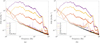 |
Figure 9 Power spectrum density of the acoustic pressures at all microphones for p0 = 2.75 bar and pf = 5.0 bar with 20 m PU tube termination (a) and closed-end termination (b). The initial gas volume is V0 = 2.00 dm3 and the final gas volume is calculated as: |

4.3 Analytical model of gas resonator impedance
Depending on the gas pressures, the gas resonator reduces the hydraulic stiffness of the system. It is assumed that the resonator walls are rigid. The water in the cavity and neck of the resonator is assumed to be incompressible. The inertia of water and piston in the cavity are neglected. The compression of gas inside the cavity is assumed to be isentropic. Viscosity losses are also neglected. A finite damping within the system is considered. This damping is used as a fit parameter in the analysis of the results. With those approximations, the impedance of the gas resonator at the junction with the main duct (neck inlet) is calculated (Appendix A) as:
 (14)
(14)
where ω0 is the resonance frequency of the undamped gas cavity and Q is the quality factor. The frequency ω0 is defined as:
 (15)
(15)
Here, leff = 12.5 mm is the effective neck length of the gas resonator and  is the ratio of specific heats at constant pressure and volume of the gas, respectively. From the fit of the measurements performed a value of Q = 1.5 was determined. The estimation of leff is provided in Appendix A.
4.4 Experimental results
Figures 9a and 9b show the power spectrum density (PSD) curves of the acoustic pressures from microphones on the source-side and transmission-side of the resonator for a 20 m PU tube termination and a closed-end termination on the transmission-side of the test-section, respectively. On the source-side, the pressure amplitudes vary linearly with distance to the inlet of the resonator (x = 0). This indicates that standing waves are dominant on the source-side of resonator. The pressure amplitudes on the source-side are four orders-of-magnitude higher than the noise floor. Hence, multi-microphone method can reliably be used to calculate the incident and the reflected wave amplitudes. It is important to note that the signal on the source side is useful in the range 1 Hz< f < 1 Hz for the source side while for the flexible-plate resonator (Fig. 3) this is only useful in the range 5 Hz < f < 300 Hz. This is beacause the source is quite different compared to setup for testing the membrane resonator. This setup has a different pump, which can reach higher flow rates and also a noisier orifice. Note furthermore the peak (f ≃ 180 Hz) in the transmission-side signals for the closed end condition (RB = −1). This is close to the quarter-wave length resonance (f = 223 Hz) of the transmission-side pipe segment (length 1.6 m).
Below the resonance frequency the pressure amplitudes on the transmission-side are above the noise floor for both terminations. For the termination with 20 m PU tube, above resonance frequency the pressure amplitudes remain close to noise-level. For the closed-end termination, the pressure amplitudes above resonance frequency are clearly above noise floor. For the closed-end termination the pressures at the microphones are generally in the order  below the quarter wave resonance frequency of 223 Hz. Hence, the measurement of TLan using multi-microphone method would be more reliable for the closed-end termination. However as it would be shown further, the robust method of calculating the TLan gives consistent results regardless of the end termination.
Figure 10 shows the comparison between the measured anechoic transmission loss (TLan) calculated using source-side multi-microphone with robust formulation, the standing wave method and the classic multi-microphone method with robust formulation for both terminations. The closed-end termination has a reflection coefficient of RB = 1. A reflection coefficient of RB = −0.8 is used for the 20 m PU tube termination [34]. As shown previously the TLan calculated using the classic multi-microphone method with robust formulation (Eq. (5)) agrees with the source-side multi-microphone and the standing-wave method over the complete frequency range. The measured TLan by the classic multi-microphone method is in fair agreement with the analytical model (at f ≤ 10 Hz). It is striking that the results are very robust and that the transmission loss curves reproduce the results for the different acoustic terminations and analysis method. This is true even close to the resonance frequency. This indicates that around the resonance frequency the measure transmission losses are meaningful. This was not the case for the flexible-plate resonator.
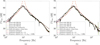 |
Figure 10 Comparison between measured TLan of the gas resonator with p0 = 3.4 bar and pf = 5.5 bar for the 20 m PU tube termination (a) and the closed-end termination (b) using the source-side multi-microphone method with robust formulation, the standing-wave method and the classic multi-microphone method with robust formulation. The measured TLan are compared to undamped analytical model, damped model with quality factor Q = 1.5 and an frequency adjusted TLan plot with Q = 1.5 and fmax = 9.0 Hz. |
Figure 11 compares the measured TLan to the TLan calculated by adjusting the maximum response frequency for both damped (Q = 1.5) and undamped cases. The TLan is calculated using the classic multi-microphone using the robust formulation for both the end terminations. The maximum response frequency (fmax) measured for the gas resonator is lower than the theoretical resonance frequency (f0) calculated by the analytical model by a maximum of 7%. When damping is not considered the adjusted frequency TLan plot agrees well with the measured TLan over most of the relevant frequency range except at the maximum response frequency. Considering a damped system with a quality factor Q = 1.5 the measured TLan plots agree with the calculated plots even at the maximum response frequency (fmax). The quality factor Q = 1.5 represents the damping within the gas resonator during the measurements. This damping could be a result of friction losses between the piston and cavity. The maximum observed transmission loss (TLmax) is in the order of 60 dB for all cases. Table 2 compares the resonance frequencies calculated from analytical model and the maximum response frequency measured for all the gas resonator configurations. The maximum TLan is also compared for the damped TLan plot and the measurements.
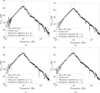 |
Figure 11 Comparison between measured, undamped frequency adjusted and damped (Q = 1.5) frequency adjusted TLan plots of the gas resonator for a 20 m long PU-tube termination (RB = −0.8) and a closed termination (RB = 1). The transmission losses were calculated using multi-microphone method with robust-formulation.The resonance frequencies are fine tuned by varying the gas volume within the resonator cavity. (a) p0 = 2.75 bar and pf = 5.0 bar; (b) p0 = 3.0 bar bar and pf = 5.5 bar bar bar; (a) p0 = 3.25 bar and pf = 5.5 bar; (a) p0 = 3.4 bar and pf = 5.5 bar. |
Comparison of resonance frequencies f0, (TLan)max and corresponding fmax for analytical undamped (Q = ∞), frequency adjusted undamped (Q = ∞) and frequency adjusted damped (Q = 1.5) from measurements.
5 Conclusions
A robust formulation (Eq. (5)) has been proposed to determine anechoic transmission losses from acoustic pressure measurements at the source and transmission side of a compact resonator placed in a water-filled pipe system. This formulation avoids the need to accurately determine the reflection coefficient RB of the setup transmission-side termination. This formulation is accurate as long as the transmission losses are large and the frequency is low enough to avoid acoustic resonance in the transmission-side pipe. Good results are obtained when combining, into this robust formulation, the classical multi-microphone method to determine the incoming wave amplitude  and the transmitted wave
  with a microphone signal
  close to the neck of the resonator as an estimate of the neck pressure pn. However, using the same multi-microphone results in the reflection coefficient formulation (Eq. (4)), results are poor. Good results are also achieved when an estimated value of RB is used to determine the transmitted-wave amplitude
  from a single microphone measurement at the transmission side. Results with RB = 1 and RB ≃ = −0.8 obtained with the robust method are equivalent. The standing-wave method allows the determination of TLan from measurements with only two microphones and is found to be reliable around the resonance frequency (for high values of TLan). It uses one source-side microphone at a reasonable distance from the resonator and a single transmission-side microphone close to the resonator neck.
The lumped element model gives a fair estimate of resonance frequencies and transmission losses for the flexible plate and gas resonators. When using the resonance frequency as a fit parameter, the magnitude of the measured anechoic transmission loss of the flexible plate resonator is within 3 dB in agreement with the analytical model, except at frequencies close to resonance. Around the resonance the transmission-side-microphone signals are below the electronic noise level. Close to the resonance frequency large deviations are observed. For the gas resonator a good fit of the measured TLan has been found by assuming that the quality factor is Q ≈ 1.5. This implies a high level of damping. This is expected to be caused by friction of the piston separating the water from the gas in the resonator cavity. For the flexible plate resonators one suspects that the transmission side pressure signals are below the electronic noise-floor around the resonance frequency. In most cases the quality factor cannot be estimated. However, a quality factor of Q ≥ 4 was estimated for the resonator with 2 mm thick plate, which is significantly higher than that of the gas resonator.
The lumped-element analytical model over-predicts the resonance frequency by about 10% for the gas resonator. The cause of the deviation in gas resonators is not clear. For the flexible-plate resonator the deviation is due to the assumptions of clamped boundary condition of the flexible plate and rigid walls of the cavity, which are not realistic for thick plates tplate ≥ 2 mm. The compliance of the aluminium-cavity side walls is important for thick plates. For thin plate tplate = 1 mm, the simple lumped model underestimates the resonance frequency. This is due the large non-linear static deformation, induced by the static pressure in the water circuit. This deformation increases the stiffness of the plate and can limit the possibility to achieve low resonance frequencies with very thin flexible plates.
The flexible-plate-resonator design is reliable, fairly compact and low-cost. The performance of the flexible-plate resonators is comparable to that of the gas resonators with equal resonance frequencies and neck length. The transmission loss of the resonators close to resonance frequencies is dependent on the effective neck length (leff). Reducing the effective neck length can improve the performance of the flexible-plate resonator. To maintain the same resonance frequency the neck diameter should also be modified, keeping  constant. Flexible plate resonators also have lower damping characteristics, which makes them ideal for low static pressure applications with high transmission losses.
Gas resonators are most suitable for low frequencies (in the present case f0 = 10 Hz). It is easier to fine-tune their resonance frequencies than for flexible-plate resonators. This is done by modifying the gas volume by varying the initial gas pressure before compression due to the increase of static pressure in the water circuit. They can be used for fluid circuits with higher static pressures than the thin flexible-plate resonators, with comparable size. They are however, more complex in design, which makes them more expensive and less robust.
Acknowledgments
The research was funded by ASML, Philips and TNO under the Flow Induced Vibrations Consortium Agreement – 20150911. The authors would like to thank ASML for providing us access to their research labs. The authors would like to give special thanks to Luuk Brummans and Ingmar Krabben for their support.
Appendix A
A.1 Lumped-element model of resonator
The flexible-plate resonator comprised a resonator cavity with a flexible plate connected to a duct by a narrow neck as a T-junction. All the resonator walls except the flexible plate are assumed rigid. The length of the cavity is assumed small compared to the acoustic wavelength and therefore the pressure in the cavity is considered to be uniform. The flow in neck is assumed to be incompressible, uniform and inviscid. The circular flexible plates on the resonators are of uniform thickness. Two models for the boundary condition of the flexible plates are presented, clamped condition and simply-supported condition. Considering uniform flow at T-junction and neglecting compressibility of the fluid, through continuity of pressure and momentum one gets:
 (A1)
(A1)
 (A2)
(A2)
where  ,
,  and pn are measured acoustic pressures on the source-side, transmission-side and the inlet of the neck, dn is the neck diameter, dp is the diameter of the pipe/duct,
  is the impedance at resonator neck. A uniform, incompressible and inviscid flow, with velocity un, is assumed in neck.The velocities are related to the acoustic wave amplitudes by
  with i = A or B. One gets from the momentum balance over the neck:
 (A3)
(A3)
where leff is the effective (acoustic) neck length (discussed in Appendix B), pc1 is the pressure in the resonator cavity. The shear stress  at the neck wall is estimated by using the thin viscous boundary layer approximation (δν ≪ dn) [6, 32]:
 (A4)
(A4)
with  the Stokes-layer thickness. Using this approximation and neglecting other frictional losses, one finds a maximum transmission loss TLan = O(80 dB). This is much higher than the observed TLmax. The viscous friction losses were therefore neglected when comparing experiments with theory.
Considering a uniform pressure in the cross-section of the cavity the surface-average velocity of the flexible plate (uc2) is calculated as:
 (A5)
(A5)
where lc is the cavity length, uc1 is the velocity at the cavity inlet and ρw is the density of water. The speed of sound cw,eff is the speed of sound in a water-filled duct calculated using the Korteweg-Lamb equation [34].
The average quasi-static velocity of the flexible plate by a uniform pressure pc1 is given by:
 (A6)
(A6)
where  is the cross-sectional area of the cavity and K is the spring constant. The spring constant for the flexible-plate resonator are given by equation (12) and for the gas resonator it is:
 (A7)
(A7)
Here the inertia of the water in the cavity and of the flexible plate (or piston) were neglected, hence the pressure  in the cavity is assumed to be uniform. This implies:
 (A8)
(A8)
Replacing value of uc2 from equation (A6) in equation (A5), neglecting friction and substituting it in equation (A3) one obtains equation (9). Since losses due to viscous effects are low. The high damping at resonance frequency implies that the transmission losses of the flexible-plate resonator around the resonance frequency cannot be measured because the pressure signal is below the detection limit. One also expects the transmission through pipe wall vibration to become dominant under these circumstances.
The losses in the gas resonator are probably dominated by the friction of the piston with the walls. This results into a relatively low quality factor. Rewriting the momentum equation (Eq. (A5)) in the form of a spring-mass-damper system:
 (A9)
(A9)
where Msys, Ksys and C are system mass, stiffness and damping. With  is the fluid displacement in the cavity and xn is the fluid displacement in the neck. One gets, Msys = ρw leff An,
  . The system damping C for gas-resonator is given by:
 (A10)
(A10)
where Q is the quality factor. Using equations (A9) and (A10), the impedance at resonator neck is calculated as:
![Mathematical equation: $$ {Z}_n=\mathrm{i}\omega {\rho }_w{l}_{\mathrm{eff}}\left[1-\frac{\mathrm{i}}{Q}\frac{{\omega }_0}{\omega }-{\left(\frac{{\omega }_0}{\omega }\right)}^2\right]. $$](/articles/aacus/full_html/2022/01/aacus220045/aacus220045-eq95.gif) (A11)
(A11)
Replacing value of Q in equation (A11) gives equation (14). The measured transmission losses for the gas resonator around the resonance frequency were quite reproducible. The quality factor Q = 1.5 estimated by visual curve fitting of the experimental data (see Figs. 10 and 11) is therefore expected to be meaningful.
Appendix B
Effective length neck
The effective neck length of the resonator is greater than the actual neck dimensions due to the inertia of the water in the neck, resonator cavity and the inertia of the moving flexible plate. Hence, effective length correction for the resonator neck is given by:
 (B1)
(B1)
Here, ln is the length of the resonator neck at the junction between duct and resonator, δn1 is the inner length correction due to transition from duct to neck in the T-junction, δn2 is the outer-length correction for the neck, δN is the length correction of the duct with diameter dN and length lN. Equations for end corrections are provided for the T-junction by Lefebvre et al. [38] and Dubos et al. [39] and for the neck-cavity transition by Kergomard and Garcia [40]. The term  corrects for the inertia of the water and the flexible plate in the resonator cavity. Here, lc is cavity length,
  is density ratio of the plate material (steel) to water. Thickness of the flexible plate is given by
  .
.
For the flexible plate resonator the inner, outer and inertial contribution of water and flexible plate to leff are calculated to be δn = 1.2 mm, δc = 2.9 mm. Since there is no duct between the neck and cavity we get lN = 0 and δN = 0. The inertial correction for the water in the cavity and flexible plate of tplate= 10 mm is  . Hence, the effective neck length is leff = 19.7 mm to 19.9 mm depending on thickness of the plate on the flexible-plate resonator.
For the gas resonator dn = 10.26 mm and thickness ln = 1.2 mm. The neck expands into a duct with diameter dN = 23 mm and length lN = 35 mm. The duct is connected to the resonator cavity with dc = 150 mm. Hence, from equation (27) the internal length correction at the T-junction is δn1 = 0.82 mm, the outer length corrections δn2 = 1.9 mm. The length correction δN = 7.8 mm is calculated using the formula of Kergomard and Garcia [40]. Hence,  . For a steel piston with tplate = 5.5 mm and s = 7.8 the calculated correction for the inertia of water and piston is 0.4 mm. Therefore one achieves the effective neck length of leff = 12.9 mm.
References
- D. Tonon, E.M.T. Moers, A. Hirschberg: Quasi-steady acoustic response of wall perforations subject to a grazing-bias flow combination. Journal of Sound and Vibration 332, 7 (2013) 1654–1673. https://doi.org/10.1016/j.jsv.2012.11.024. [CrossRef] [Google Scholar]
- L. Hu, Y. Shi, Q. Yang, G. Song: Sound reduction at a target point inside an enclosed cavity using particle dampers. Journal of Sound and Vibration 384 (2016) 45–55. https://doi.org/10.1016/j.jsv.2016.08.016. [CrossRef] [Google Scholar]
- R. Aslan, O. Turan: An acoustic structure design supported by shear thickening fluid for sound absorption. Applied Acoustics 182 (2021) 108–257. https://doi.org/10.1016/j.apacoust.2021.108257. [CrossRef] [Google Scholar]
- U. Ingard, V.K. Singhal: Effect of flow on the acoustic resonances of an open – ended duct. The Journal of the Acoustical Society of America 58, 4 (1975) 788–793. https://doi.org/10.1121/1.380751. [CrossRef] [Google Scholar]
- D. Bechert: Sound absorption caused by vorticity shedding, demonstrated with a jet flow. Journal of Sound and Vibration 70, 3 (1980) 389–405. https://doi.org/10.1016/0022-460X(80)90307-7. [CrossRef] [Google Scholar]
- P. Morse, U. Ingard: Theoretical Acoustics. Princeton University Press, 1986. ISBN: 9780691024011. [Google Scholar]
- M.S. Howe: Damping of sound and vibration by flow nonlinearity in the apertures of a perforated elastic screen. IMA Journal of Applied Mathematics 55, 3 (1995) 221–242. https://doi.org/10.1093/imamat/55.3.221. [CrossRef] [Google Scholar]
- G. Hofmans, R. Boot, P. Durrieu, Y. Auregan, A. Hirschberg: Aeroacoustic response of a slit-shaped diaphragm in a pipe at low Helmholtz number, 1: Quasi-steady results. Journal of Sound and Vibration 244, 1 (2001) 35–56. https://doi.org/10.1006/jsvi.2000.3457. [CrossRef] [Google Scholar]
- D. Zhao, X.Y. Li: A review of acoustic dampers applied to combustion chambers in aerospace industry. Progress in Aerospace Sciences 74 (2015) 114–130. https://doi.org/10.1016/j.paerosci.2014.12.003. [CrossRef] [Google Scholar]
- Z. Zuti, C. Shuping, W. Huawei, L. Xiaohui, D. Jia, Z. Yuquan: The approach on reducing the pressure pulsation and vibration of seawater piston pump through integrating a group of accumulators. Ocean Engineering 173 (2019) 319–330. https://doi.org/10.1016/j.oceaneng.2018.12.078. [CrossRef] [Google Scholar]
- B. Liu, L. Yang: Transmission of low-frequency acoustic waves in seawater piping systems with periodical and adjustable Helmholtz resonator. Journal of Marine Science and Engineering 5 (2017) 4. https://doi.org/10.3390/jmse5040056. [CrossRef] [Google Scholar]
- K.L. Coakley: Bellows accumulators for 8000 psi hydraulic systems, in Aero. Tech. Conf. Expos., SAE International, 1985. https://doi.org/10.4271/851914. [Google Scholar]
- G. Hu, L. Tang, X. Cui: On the modelling of membrane-coupled Helmholtz resonator and its application in acoustic metamaterial system. Mechanical Systems and Signal Processing 132 (2019) 595–608. https://doi.org/10.1016/j.ymssp.2019.07.017. [CrossRef] [Google Scholar]
- M.H. Kurdi, G. Scott Duncan, S.S. Nudehi: Optimal design of a Helmholtz resonator with a flexible end plate. The Journal of Vibration and Acoustics 136 (2014) 3. https://doi.org/10.1115Z1.4026849. [CrossRef] [Google Scholar]
- S.S. Nudehi, G.S. Duncan, U. Farooq: Modelling and experimental investigation of a Helmholtz resonator with a flexible plate. The Journal of Vibration and Acoustics 135 (2013) 4. https://doi.org/10.1115/1.4023810. [CrossRef] [Google Scholar]
- W. Frommhold, H. Fuchs, S. Sheng: Acoustic performance of membrane absorbers. Journal of Sound and Vibration 170, 5 (1994) 621–636. https://doi.org/10.1006/jsvi.1994.1091. [Google Scholar]
- M. Kurdi, S. Nudehi, G.S. Duncan: Tailoring plate thickness of a Helmholtz resonator for improved sound attenuation, in Ser. Int. Design Eng. Techn. Conf. Comput. Inf. Eng. Conf. 8: 28th Conf. Mech. Vib. Noise, Aug. 2016. https://doi.org/10.1115/DETC2016-59302. [Google Scholar]
- M. Khairuddin, M. Said, A. Dahlan, K. Kadir: Review on resonator and muffler configuration acoustics. Archives of Acoustics 43 (2018) 3. [Google Scholar]
- C. Cai, C.M. Mak: Acoustic performance of different Helmholtz resonator array configurations. Applied Acoustics 130 (2018) 204–209. https://doi.org/10.1016/j.apacoust.2017.09.026. [CrossRef] [Google Scholar]
- D. Wu, N. Zhang, C.M. Mak, C. Cai: Hybrid noise control using multiple Helmholtz resonator arrays. Applied Acoustics 143 (2019) 31–37. https://doi.org/10.1016/j.apacoust.2018.08.023. [CrossRef] [Google Scholar]
- M.L. Munjal, A.G. Doige: Theory of a two source-location method for direct experimental evaluation of the four-pole parameters of an aeroacoustic element. Journal of Sound and Vibration 141, 2 (1990) 323–333. https://doi.org/10.1016/0022-460X(90)90843-0. [CrossRef] [Google Scholar]
- S. Griffin, S.A. Lane, S. Huybrechts: Coupled Helmholtz resonators for acoustic attenuation. The Journal of Vibration and Acoustics 123, 1 (2000) 11–17. https://doi.org/10.1115Z1.1320812. [Google Scholar]
- M. Oblak, M. Pirnat, M. Boltezar: An impedance tube submerged in a liquid for the low-frequency transmission-loss measurement of a porous material. Applied Acoustics 139 (2018) 203–212. https://doi.org/10.1016/j.apacoust.2018.04.014. [CrossRef] [Google Scholar]
- J. Gong, Z. Jiang, L. Xuan, B. Ying, W. Peng: Numerical analysis of the transmission loss of water Muffler according to the two-load method. Proc. Inst. Mech. Eng., Part C: J. Mech. Eng. Sci. 234, 20 (2020) 3982–3991. https://doi.org/10.1177/0954406220919464. [CrossRef] [Google Scholar]
- H. Ortwig: Experimental and analytical vibration analysis in fluid power systems. Int. J. Solids Struct. 42, 21 (2005) 5821–5830. https://doi.org/10.1016/j.ijsolstr.2005.03.028. [CrossRef] [Google Scholar]
- H.H. Hubdard: Aeroacoustics of flight vehicles: theory and practice, Vol 2: Noise Control, NASA, 1991. [Google Scholar]
- S. Allam, M. Abom: Investigation of damping and radiation using full plane wave decomposition in ducts. Journal of Sound and Vibration 292, 3 (2006) 519–534. https://doi.org/10.1016/j.jsv.2005.08.016. [CrossRef] [Google Scholar]
- J. Golliard, Y. Auregan, T. Humbert: Experimental study of plane wave propagation in a corrugated pipe: Linear regime of acoustic-flow interaction. Journal of Sound and Vibration 472 (2020) 115158. https://doi.org/10.1016/j.jsv.2019.115158. [CrossRef] [Google Scholar]
- M. Junger, D. Feit: Sound, structures, and their interaction. MIT Press, 1972. [Google Scholar]
- M. Prek: Wavelet analysis of sound signal in fluid-filled viscoelastic pipes. The Journal of Fluids 19, 1 (2004) 63–72. https://doi.org/10.1016/j.jfluidstructs.2003.09.003. [Google Scholar]
- M. Munjal: Ducts and Mufflers. John Wiley & Sons, 1987. ISBN 0-471-84738-0. [Google Scholar]
- M.J. Lighthill: Waves in Fluids. Cambridge University Press, 1978. ISBN 0521292336. [Google Scholar]
- S.H. Jang, J.G. Ih: On the multiple microphone method for measuring in-duct acoustic properties in the presence of mean flow. Journal of the Acoustical Society of America 103, 3 (1998) 1520–1526. https://doi.org/10.1121/1.421289. [CrossRef] [Google Scholar]
- C.M.J. Moonen, N.P. Waterson, N.R. Kemper, D.M.J. Smeulders: Experimental study of resonance in water circuit with mixed rigid and flexible hosing, in Proc. 11th Int. Conf. Flow-Ind. Vib., The Hague, The Netherlands: FIV, 2016. [Google Scholar]
- S. Timoshenko, S. Woinowsky-Krieger: Theory of plates and shells (Engineering Mechanics Series). McGraw-Hill, 1959. [Google Scholar]
- W.C. Young, R.G. Budynas: Roark’s Formulas for Stress and Strain. McGraw-Hill Education, 2001. [Google Scholar]
- R.H. Plaut: A generalized Reissner theory for large axisymmetric deflections of circular plates. Journal of Applied Mechanics 81 (2013) 3. https://doi.org/10.1115/1.4024413. [Google Scholar]
- A. Lefebvre, G.P. Scavone: Characterization of woodwind instrument toneholes with the finite element method. Journal of the Acoustical Society of America 131, 4 (2012) 3153–3163. https://doi.org/10.1121/1.3685481. [CrossRef] [PubMed] [Google Scholar]
- V. Dubos, J. Kergomard, A. Khettabi, J. Dalmont, D. Keefe, C. Nederveen: Theory of sound propagation in a duct with a branched tube using modal decomposition. Acta Acustica united with Acustica 85 (1999) 153–169. https://doi.org/10.1016/j.apacoust.2017.09.026. [Google Scholar]
- J. Kergomard, A. Garcia: Simple discontinuities in acoustic waveguides at low frequencies: Critical analysis and formulae. Journal of Sound and Vibration 114, 3 (1987) 465–479. https://doi.org/10.1016/S0022-460X(87)80017-2. [CrossRef] [Google Scholar]
Cite this article as: Kottapalli S. van de Meerendonk R. Waterson N. Nakiboglu G. Hirschberg A, et al. 2022. Analytical modelling and experimental validation of compliance-based low-frequency resonators for water circuits. Acta Acustica, 6, 56.
All Tables
Comparison of resonance frequencies of the flexible-plate resonator with different plate thicknesses using analytical model, finite-element model (FEM) and experiments.
Comparison of resonance frequencies f0, (TLan)max and corresponding fmax for analytical undamped (Q = ∞), frequency adjusted undamped (Q = ∞) and frequency adjusted damped (Q = 1.5) from measurements.
All Figures
|
Figure 1 Schematic of the test-section and detailed view of the resonator neck. (a) Schematic of the experimental setup with source-side microphones (A1, A2, A3, A4) and transmission-side microphones (B1, B2, B3, B4). The entire flow system is the broadband noise source. There is no steady flow along the resonator in the main duct. (b) Schematic of the T-junction between the neck of the resonator and the main duct. The termination of the transmission side of the main pipe is either a closed end at the end of the steel tube (with closed ball-valve 1) or the PU tube termination (with closed ball-valve 2). |
| In the text | |
|
Figure 2 Diagram and dimensions of the flexible-plate resonator. (a) Internal dimensions of flexible-plate resonator. (b) A parallel-perspective view of the resonator. |
| In the text | |
|
Figure 3 Power spectrum density plots of acoustic pressures measured at source-side (solid lines) and transmission-side microphones (dashed lines) of flexible-plate resonator with tplate = 2 mm for (a) the 45 m PU tube termination and (b) the closed-end termination on the transmission-side. At the resonance frequency of 37 Hz, the transmitted signal is close to the noise floor. |
| In the text | |
|
Figure 4 Comparison of measured TLan calculated using source-side multi-microphone, classic multi-microphone method with robust and reflection-coefficient dependent formulation, and the standing-wave method for flexible-plate resonator with tplate = 2 mm for (a) the 45 m PU-tube (RB = −0.8) termination, and (b) the closed-end termination (RB = 1) on the transmission-side. The effect of error in the estimated reflection coefficient RB on measured TLan is shown in (c). |
| In the text | |
|
Figure 5 Comparison between measured TLan of a dynamically isolated test setup and a rigidly connected test setup to the sound source (orifice). The TLan was calculated using the multi-microphone method for flexible plate resonator with tplate = 1 mm (a) and 2 mm (b). |
| In the text | |
|
Figure 6 Comparison between measured, analytically estimated and FEM estimated TLan of flexible plate resonators with tplate = 1 mm (a), 2 mm (b), 3 mm (c), 4 mm (d) and 10 mm (e). The measured TLan have been calculated using the multi-microphone method for both terminations. The adjusted frequency fit TLan value is estimated from a visually guess of the maximum response frequency fmax from the measurements. |
| In the text | |
|
Figure 7 Cross-sectional view of of the gas resonator. Gas in the gas-cavity is separated from the water in the water-cavity by a free moving piston attached to a bellow. |
| In the text | |
|
Figure 8 Operation procedure of the gas resonator. The gas-cavity is is initially filled with air at absolute pressure p0 by using a gas inlet valve on top of the resonator without any static pressure from fluid circuit, hence gas-cavity has initial volume V0. Once the pressure in the water circuit is increased up to the final pressure pf the volume of the gas-cavity reduces from V0 to Vf. |
| In the text | |
|
Figure 9 Power spectrum density of the acoustic pressures at all microphones for p0 = 2.75 bar and pf = 5.0 bar with 20 m PU tube termination (a) and closed-end termination (b). The initial gas volume is V0 = 2.00 dm3 and the final gas volume is calculated as: |
| In the text | |
|
Figure 10 Comparison between measured TLan of the gas resonator with p0 = 3.4 bar and pf = 5.5 bar for the 20 m PU tube termination (a) and the closed-end termination (b) using the source-side multi-microphone method with robust formulation, the standing-wave method and the classic multi-microphone method with robust formulation. The measured TLan are compared to undamped analytical model, damped model with quality factor Q = 1.5 and an frequency adjusted TLan plot with Q = 1.5 and fmax = 9.0 Hz. |
| In the text | |
|
Figure 11 Comparison between measured, undamped frequency adjusted and damped (Q = 1.5) frequency adjusted TLan plots of the gas resonator for a 20 m long PU-tube termination (RB = −0.8) and a closed termination (RB = 1). The transmission losses were calculated using multi-microphone method with robust-formulation.The resonance frequencies are fine tuned by varying the gas volume within the resonator cavity. (a) p0 = 2.75 bar and pf = 5.0 bar; (b) p0 = 3.0 bar bar and pf = 5.5 bar bar bar; (a) p0 = 3.25 bar and pf = 5.5 bar; (a) p0 = 3.4 bar and pf = 5.5 bar. |
| In the text | |
Current usage metrics show cumulative count of Article Views (full-text article views including HTML views, PDF and ePub downloads, according to the available data) and Abstracts Views on Vision4Press platform.
Data correspond to usage on the plateform after 2015. The current usage metrics is available 48-96 hours after online publication and is updated daily on week days.
Initial download of the metrics may take a while.