| Issue |
Acta Acust.
Volume 6, 2022
|
|
|---|---|---|
| Article Number | 60 | |
| Number of page(s) | 18 | |
| Section | Nonlinear Acoustics, Macrosonics | |
| DOI | https://doi.org/10.1051/aacus/2022056 | |
| Published online | 22 December 2022 | |
Scientific Article
Identification of the parameters of a simplified 2 degree of freedom model of a nonlinear vibroacoustic absorber coupled to an acoustic system in linear and nonlinear forced regimes
1
LA2MP, ENIS, Km 4 Route de la Soukra, Sfax 3038, Tunisia
2
Aix Marseille Univ, CNRS, Centrale Marseille, LMA, 4 impasse Nikola Tesla CS40006, 13453 Marseille Cedex 13, France
* Corresponding author: This email address is being protected from spambots. You need JavaScript enabled to view it.
Received:
21
July
2022
Accepted:
22
November
2022
Abstract
This article presents a method for identifying the parameters of a simplified 2 degree of freedom model representative of a linear primary system coupled to a non-linear absorber in a forced harmonic regime over a wide range of amplitudes and forcing frequencies covering different dynamical regimes. This is a priori a difficult operation because it is necessary to combine two apparently contradictory steps. The first step consists in establishing models representing the physics of the system which are analytically soluble, which imposes severe approximations. The second step consists in adjusting the parameters of the models to experimental data, which reveal some phenomena ignored by the models. To do so, two approximate analytic methods, Harmonic Balance and Complexification Averaging under 1:1 resonance, are used to describe the dynamics of the nonlinear system for its different operating regimes: linear behavior, nonlinear behavior without energy pumping, energy pumping, and saturation regime. Then, using a non-linear regression, the parameters of the simplified model are identified from experiments. The values obtained correspond to the expected physical quantities.
Key words: Noise reduction / Energy pumping / Nonlinear vibroacoustic absorber / Nonlinear identification
© The Author(s), Published by EDP Sciences, 2022
 This is an Open Access article distributed under the terms of the Creative Commons Attribution License (https://creativecommons.org/licenses/by/4.0), which permits unrestricted use, distribution, and reproduction in any medium, provided the original work is properly cited.
1 Introduction
Vibroacoustic Nonlinear Energy Sinks (NES) are mechanical absorbers that are used for passive noise and vibration control in the low frequency range. Under certain conditions (related to the initial conditions and the excitation level), these absorbers lead to the phenomenon of energy pumping. This phenomenon can be defined as the unidirectional and irreversible transfer of vibrational energy from the primary system to be controlled to the auxiliary non-linear oscillator. This phenomenon is also called Targeted Energy Transfer and was originally introduced by O. Gendelman and A. Vakakis [1, 2] in the field of mechanical vibrations.
In the acoustic field the first work that experimentally showed the presence of the energy pumping phenomenon was proposed by Cochelin et al. [3]. In this paper a non-linear passive vibroacoustic absorber which was constituted by a thin circular viscoelastic membrane was developed. This viscoelastic membrane, when vibrating under very high amplitude, showed a strongly non-linear behavior, which could be described as a non-linear mass/stiffness/nonlinear damping dynamic system. The proposed experimental setup allowed to control an acoustic field in the vicinity of the first acoustic mode of a tube open at both ends. This tube was coupled to the NES through a coupling box and was excited by a loudspeaker. This experimental set-up was improved by Bellet et al. [4]. In this paper different experimental results were presented: behavior under harmonic excitation, free oscillations and frequency responses. For different excitation amplitudes, several types of frequency response have been observed (linear behavior, non-linear behavior without energy pumping, energy pumping and saturation regime). A simplified 2 degrees of freedom (DOF) model was developed and validated by a comparison between numerical calculation and experimental results. It was shown that the use of different membranes mounted in parallel on the coupling box extended the efficiency range of the energy pumping phenomenon. A second experimental acoustic energy pumping device was developed by Mariani et al. [5]. This device consisted of a diaphragm of a loudspeaker whose mass could be precisely adjusted and coupled with the primary acoustic medium to be controlled (again the first acoustic mode of an open-ended tube) through a coupling box. In these papers [3–6], the NES was linked to the primary system by a linear stiffener whose stiffness could be adjusted by controlling the volume of the coupling box.
Shao et al. [7] analyzed the energy pumping for another configuration where a vibroacoustic NES is directly linked to the primary system. In this configuration, the primary system was a parallelepipedic acoustic cavity excited in one of its modes and the NES was always a membrane mounted on one of the surfaces of this cavity. To generalize the results found in [7], J. Shao studied this system where several acoustic modes of the parallelepipedic cavity are taken into account [8]. The experimental set-up described in [9] allowed to present the energy pumping between this cavity and the membrane.
Recently, a purely acoustic non-linear absorber has been developed based on a Helmholtz resonator. It has been shown experimentally that under certain conditions this device can exhibit a non-linear behavior [10, 11]. The non-linear behavior of this absorber has been studied analyticly, numerically and experimentally [12]. Energy pumping between an acoustic medium and the Helmholtz nonlinear resonator has been studied by Gourdon et al. [13].
For the modeling of these systems, the authors have imposed simplifications. In [4], to obtain the equations governing the coupled tube-membrane system, R. Bellet assumed that the spatial dependence of the acoustic pressure inside the tube was described by the first eigenmode of a tube open at both ends and that the displacement imposed on the membrane had a parabolic shape.
For a wide range of amplitudes and frequencies, this simplification is crude. In any case, the pressure model is only valid in the immediate frequency vicinity of the corresponding mode; similarly, the parabolic shape imposed on the membrane displacement is only valid when the membrane vibrates with a very low amplitude. These approximations are made at the expense of the accuracy of the model. As pointed out by Bellet et al. [4], the agreement between the simplified model and the experiments could not be obtained over the whole range of amplitudes and frequencies with a single set of parameters. In fact, raises questions on the model about its domain of validity and the identification of its parameters.
In this paper we have sought to correct the inherent inaccuracy of the model by allowing the parameters of the system to vary with the excitation amplitude. In a way, this is equivalent to allowing additional degrees of freedom that can vary with the excitation amplitude. These parameters are: force, pulsation and linear stiffness of the tube, linear and non-linear stiffness and dissipation of the diaphragm, coupling term and the mass term. The interest of this approach, apart from the fact that it allows the continued use of a simplified model that allows relatively simple analytic developments, also lies in a better understanding of the physics underlying the phenomena. The observed variations of the identified parameters will make it possible to identify the points to be refined in the modeling or estimate a range of validity of constant parameters.
The identification of the parameters of a nonlinear model has been practiced for long with many different approaches. To cite only a few, there is the application of Nayfeh’s multiple time-scale approach [14], the classical use of a minimization algorithm on a simple model [15] or on a black-box system representation [16]. Neural networks are also used [17], and systems can be represented with Kalman filters [18]. In all these previous works the authors identify the parameters of models of nonlinear dynamical systems, but to the best of our knowledge the method we present here has not yet been used. These parameters are the minimum set of independent parameters that was found necessary to describe the complex dynamics of the system under study [4]. In order to be able to identify the parameters of this 2 DOF model over a wide range of forcing amplitudes, we tested two different ways to obtain simple analytic expressions to describe the nonlinear dynamics of the system: Harmonic Balance Method [19–21] denoted in the following HBM and Manevitch Complexification Averaging method [22] denoted in the following CX-A method. Using a non-linear regression, the parameters of the simplified model were identified from experiments. It should be noted that the principles of this identification method can be applied to any non-linear differential system with a low number of degrees of freedom that describes the coupling between a primary system and a NES.
This article is organised as follows. In the second part, an experimental description of the fixture is presented. The simplified adimensional model of R. Bellet is presented and the model adapted to our problem is deduced. In the third part, the identification method is described: we describe in detail the experimental tests carried out and then we establish the two expressions of the identification functions which describe the dynamics of the nonlinear system resulting from the HBM and CX-A and we describe the nonlinear regression that is used. In the fourth part, the result of the identification is presented. We compare the experimentally determined frequency responses with those given from the identification using the HBM and CX-A. The ridge curves from the identified parameters and by using the experimentally determined parameters at low excitation amplitude are compared with the ridge curve given from the sound pressure measurement in the tube. The time responses of the system calculated numerically from the parameters identified by using the HBM and CX-A are compared with the experimental data. The estimated variation of the parameters of our system as a function of the excitation amplitude in the two domains (linear and non-linear) is presented. This method is applied to other experimental configurations 1. Finally, the last part concludes this paper.
2 Description of the system under study
2.1 Description of the experimental set-up
The device is inspired by the work of Cochelin et al. [3] and Bellet et al. [4]. The non-linear vibroacoustic absorber (NES) is always constituted by a thin circular viscoelastic membrane which is subjected to an axisymmetric transverse displacement which is the source of the non-linearity. This absorber is coupled to the first resonance mode of an open tube through a coupling box. The primary tube system is excited by an acoustic field provided by a loudspeaker (see Fig. 1). In this work, the dimensions of the tube and the coupling box are fixed. The radius of the tube is Rt = 0.045 m, its length is Lt = 2.2 m, its first resonant frequency is ft = 79 Hz. The volume of the coupling box is Vc = 29.3l. The membrane of variable thickness hm and variable radius Rm is fixed to the coupling box by means of a holder which allows the change of the diameter and the tension exerted on the membrane. In the range of frequencies and levels we have worked, the z shape of the tube has no meaningful effect on the acoustic phenomena. For the three series of experimental tests carried out, the same tube was kept and the membrane was changed each time. The three configurations are:
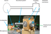 |
Figure 1 Experimental fixture. |
 |
Figure 2 schematic diagram of the experimental set-up and equivelent mechanical representation. |
Configuration 1: hm1 = 0.23 mm, Rm1=5 cm, fm1 = 45 Hz.
Configuration 2: hm2 = 0.24 mm, Rm2=4 cm, fm2 = 44 Hz.
Configuration 3: hm3 = 0.62 mm, Rm3=5 cm, fm3 = 45 Hz.
The voltage sent to the amplifier must not exceed 1.75 V in order to avoid to damage the loudspeaker. For the first and second experiments, the maximum voltage sent to the amplifier is equal to 1.75 V and 0.75 V. These levels of excitation are higher than those of energy pumping, and we observed the saturation of the membrane. In the third experiment we reached the maximum voltage that we can apply (1.75 V), without seeing the end of the energy pumping and the saturation of the membrane.
2.2 Experimental tests
First, a series of experimental tests were carried out on the experimental fixture presented in the Figure 1. This series of experimental tests is automated through a program written on Matlab that allows the acquisition system (NetdB) to be driven directly through the TCP/IP communication mode. This acquisition system has twelve synchronous acquisition channels and two signal generation channels with a sampling frequency fixed for all experiments at 12.8 kHz. The setup allows the tube to be excited by a harmonic acoustic field through a loudspeaker. The loudspeaker is fed through a TIRA 120BBA amplifier whose input signal is provided by the NetdB acquisition system. A low-pass filter with a bandwidth of [0,1000] Hz filters the output signal of NetdB in order to avoid polluting the excitation signals with noise. An amplitude-frequency excitation range has been defined for each type of arrangement. The frequency steps of 0.4 Hz and voltage steps of 0.01 V are a compromise between the fineness of analysis sufficient to describe the whole response range of the system and the measurement time; it was chosen not to have a total acquisition time greater than 3 days to ensure relative stability of the experimental conditions.
A Keyence LK-G152 laser displacement sensor, connected to a Keyence LK-G3001 controller, measures the displacement of the centre of the membrane. The measurement range of this displacement sensor is ±40 mm. The sensitivity setting for this sensor is set to 102 v/m.
A GRAS 46BF microphone with a sensitivity of 3.6 mv/Pa measures the acoustic pressure in the middle of the tube; from this pressure measurement, the value of the displacement at each point of the acoustic medium can be deduced by the conservation equations. A GRAS 46DP type microphone with a sensitivity of 0.9 mv/Pa measures the acoustic pressure in the coupling box on the loudspeaker side; from this measurement we can estimate the forcing term F corresponding to each excitation voltage sent to the loudspeaker terminal. The location of the microphones and the displacement sensor are shown in Figure 1.
Three NetdB input channels are used to monitor the voltage sent by the NetdB signal generator to the TIRA amplifier, the voltage and the current output of the TIRA amplifier. These three measurements are a means of monitoring and verifying that our series of experimental tests is running smoothly. The procedure is to start recording at t0 = 0 s. At t1 = 1.25 s the signal is sent to the speaker for 10 s. The system rests for 1 s and then the recording stops. A further two seconds of waiting is added, in order to allow the data to be transferred from the data acquisition chain to the PC controlling the measurement. The Root Mean Square (RMS) of the last three seconds of the signal (before the source is switched off) is calculated so as to estimate the steady state value. This allows the RMS amplitude frequency responses of the air in the tube and the membrane to be determined. An example of the amplitude–frequency response surface of the tube displacement UExp and the membrane displacement QExp are shown in Figure 3. These results correspond to the first membrane configuration: hm = 0.23 mm, Rm = 5 cm, fm = 45 Hz.
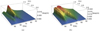 |
Figure 3 Experimentally determined amplitude-frequency response surfaces of the tube (a) and membrane (b) for configuration 1: hm = 0.23 mm, Rm = 5 cm, fm = 45 Hz. |
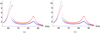 |
Figure 4 Normalized frequency responses of the membrane determined analyticly (red) and experimentally (blue). (a) maximum analytic solution (b) minimum analytic solution. |
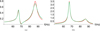 |
Figure 5 Normalized results of identification (V = 0.01 V). Blue: identification using HBM. Green: CX-A method. Red: experimental frequency response functions. (a) tube displacement, (b) membrane displacement. Configuration 1: hm = 0.23 mm, Rm = 5 cm, fm = 45 Hz. |
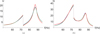 |
Figure 6 Normalized results of identification (V = 0.27 V). Blue: identification using HBM. Green: CX-A method. Red: experimental frequency response functions. Gray dots: discontinuity, guide to the eye. (a) tube displacement, (b) membrane displacement. Configuration 1: hm = 0.23 mm, Rm = 5 cm, fm = 45 Hz. |
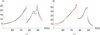 |
Figure 7 Normalized results of identification (V = 0.52 V). Blue: identification using HBM. Green: CX-A method. Red: experimental frequency response functions. Gray dots: discontinuity, guide to the eye. (a) tube displacement, (b) membrane displacement. Configuration 1: hm = 0.23 mm, Rm = 5 cm, fm = 45 Hz. |
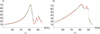 |
Figure 8 Normalized results of identification (V = 1.12 V). Blue: identification using HBM. Green: CX-A method. Red: experimental frequency response functions. Gray dots: discontinuity, guide to the eye. (a) tube displacement, (b) membrane displacement. Configuration 1: hm = 0.23 mm, Rm = 5 cm, fm = 45 Hz. |
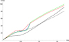 |
Figure 9 Ridge curves of U (maximum amplitudes over all frequency range). Red: normalized experimental data. Blue: numerical integration of the equations with parameters identified by HBM. Green: numerical integration with parameters identified by CX-A. Continuous black: numerical integration with parameters determined experimentally at low excitation amplitude. Dashed black: numerical intergration with the mean parameters determined by HBM inside the pumping zone. Configuration 1: hm = 0.23 mm, Rm = 5 cm, fm = 45 Hz. |
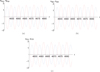 |
Figure 10 Time series of the two degrees of freedom of the system. f = 85 Hz, V = 0.025 V. The blue curves show the scaled displacement of the air at the end of the tube and the red curves show the scaled displacement at the center of the membrane. Top left: measured time responses. Top right: the numerically determined time responses using the parameters identified from the HBM. Bottom: the temporal responses determined numerically using the parameters identified from the CX-A method. Configuration 1: hm = 0.23 mm, Rm = 5 cm, fm = 45 Hz. (a) The measured time responses. (b) The numerically determined time responses using the parameters identified from the HBM. (c) The numerically determined time responses using the parameters identified from the CX-A method. |
3 Identification method
3.1 Simplified system model
The model of this coupled tube-membrane system used here was established by Bellet et al. [4]. We present here only the final model because the full derivation would distract the reader from the main point. A representation of the system is seen in Figure 2. It consists of a double Rayleigh-Ritz reduction of the conservation equations of the coupled tube/membrane system: the acoustic field is assumed to be described by the first acoustic mode of the tube and the deformation of the membrane is approximated by an axisymmetric parabolic deformation.
In order to find the model used in this work and represented in the figure, we start from the adimensionalized dynamical model [4]
 (1)
(1)
where u and q are the normalised displacements of the air at the end of the tube and at the centre of the membrane, λ and c1ηωt the linear damping coefficients, 2c2ηωt the non-linear damping coefficient, ωt the tube resonance pulsation, F the forcing amplitude, Ω the excitation pulsation, β the coupling term, γ the dynamic mass, c1 (1 − χ) and c3 the linear and cubic stiffnesses of the membrane, χ the coefficient of pre-stress of the membrane, and η is a parameter that characterizes the membrane damping.
We propose to simplify this model in order to remove the linear dependencies between the initial parameters, and be able to fit meaningful parameters only. In previous works the two coefficients c1 and c3 were used [4] but we show here as a side result that the use of only one of those is enough. c1 and c3 are  and
and  [4]. It is worth noting that
  then c1 ≃ c3. We can therefore rewrite the system in the following form
 (2)
(2)
where kl = c1(1 − χ) and knl = c1 are the linear and non-linear stiffnesses of the membrane, ωtcη is the damping coefficient of the membrane where cη = c1η. Note that here the same coefficient is used to describe both the linear damping ωtcη and the non-linear damping 2ωtcη.
In this model is related to the simplified representation in Figure 2 by the following equations:  ;
;  .
.
The relationship between the normalized displacements (u, q) and the physical ones (up, qp) are
 (3)
(3)
For the configuration 1 we get u = 7360up and q = 4550qp.
3.2 Determination of the system parameters in linear regime
The dimensions of the tube, the membrane and the coupling box were determined by static measurements. These measurements were used to calculate the stiffness and mass terms. A dynamic measurement with a generator and an oscilloscope was made in order to determine the frequencies at the maximum amplitude of the tube and the membrane, and the frequency bands at −3 dB of the maximum amplitude. Through this dynamic measurement, where the behavior of the system is purely linear, the dissipation terms of the tube and membrane were determined. The values of these parameters are used later in the inversion procedure and as a verification tool at low excitation amplitude. We obtained the following values for F = 0.3: λ = 0.0461 s, β = 0.0874, γ = 0.170 s−2, kl = 0.0558, cη = 40 · 10−9,ωt = 496 rad/s). This process gives an estimation of all the linear parameters. Among the model parameters in equation (2), it only misses the nonlinear stiffness of the membrane. This identification method was shown to give inaccurate results at high amplitudes [4] where the nonlinear terms become meaningful.
3.3 The identification functions describing the movement of the membrane and the air at the end of the tube
In order to find analytic expressions describing the coordinates of the system, we need to solve our system of nonlinear differential equations equation (1), which is impossible in general without approximations. We will apply two analytic methods widely used for the study of non-linear dynamic systems, the HBM and the Manevitch CX-A method under 1:1 resonance. These analytic methods make it possible to highlight the influence of the various parameters of the system. The hypotheses and the full description of these methods are out of the scope of this paper. One only needs to know that in this study, HBM gives a harmonic approximate solution, and CX-A a periodic one but not necessarily harmonic. The CX-A method is more complex but it is able to describe the strongly modulated responses seen in Figure 11, which HBM cannot do, thus it is interesting to compare results obtained by these two methods.
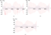 |
Figure 11 Time series of the two degrees of freedom of the system. f = 85 Hz, V = 0.61 V. The blue curves show the scaled displacement of the air at the end of the tube and the red curves show the scaled displacement at the centre of the membrane. Top left: measured time responses. Top right: the numerically determined time responses using the parameters identified from the HBM. Bottom: the temporal responses determined numerically using the parameters identified from the CX-A method. Configuration 1: hm = 0.23 mm, Rm = 5 cm, fm = 45 Hz. (a) Measured time responses. (b) The numerically determined time responses using the parameters identified from the HBM. (c) The numerically determined temporal responses using the parameters identified from the CX-A method. |
3.3.1 Identification function obtained by the harmonic balance method
Harmonic balancing is a frequency method which consists in writing the coordinates of our system in a Fourier series. In our case we will limit ourselves to the first harmonic where the coordinates of the problem are expressed in the form u(τ) = UHB cos(ωτ − ϕt) and q(τ) = QHB cos(ωτ − ϕm). By replacing these expressions in the systyem equation (2) and  by ω and neglecting the higher order harmonics, we obtain the system of algebraic equations
 (4)
(4)
The application of the harmonic balance on the system of equations (4) leads to the system of equations


 (5)
(5)
where  ,
,  , cHB = β − ω2 + 1 and d = λω.
By multiplying the first two equations of the system equation (5) by β and substituting βUcos(ϕt) and βUsin(ϕt) by their expressions given by the last two equations we obtain the system of equations equation (6)

 (6)
(6)
By simple calculation and by replacing aHB, bHB, cHB and dHB by their expressions we obtain the two equations which relate the amplitudes of oscillation of the displacements to the parameters of the model

 (7)
(7)
where αHBi and βHBi with i = 1, 2, 3 are defined as:


 (8)
(8)
The system of equation (7) is composed by two third degree polynomials of  . The coefficients of the first equation depend only on the parameters of the system and the forcing. The second equation calculates the displacement of the air in the tube UHB as a function of the displacement of the membrane QHB. The first equation is therefore solved first and then the solution of the second equation is determined.
The first third degree polynomial of  has three solutions. The type of these roots depends on the sign of the discriminant of the polynomial Δ. Recall that the discriminant of a third degree polynomial P(x) = ax3 + bx2 + cx+d is given by ΔP = b2c2 + 18abcd − 27a2d2 − 4ac3 − 4b3d. If Δ > 0 we have three distinct real roots. If Δ < 0 we have one real root and two non-real conjugate complex roots. If Δ = 0 we have a double or triple root. In this case one seeks from these three roots Q1, Q2 and Q3 a function which describes the displacement of the membrane according to the parameters of the system where one will sort out for each combination of the parameters the root which describes the stable behavior of the membrane.
Firstly, we construct a function called Sig which allows us to distinguish between real and complex roots. It is defined by
Sig: QHB → Sig(QHB)
QHB → 1 if QHB is purely real
−1 if QHB is complex.
In the case where the three roots are real, i.e. {Sig(Q1), Sig(Q2), Sig(Q3)} = {1, 1, 1}, the solution describing the displacement of the membrane corresponds to the minimal solution QHB = min{Q1, Q2, Q3}. This choice is adopted in order to present a peak of the curve that corresponds better to the experimental data. All the experiments started with null initial conditions, so the system reached only the lowest stable response after the transients. Figure 4 shows the frequency responses of the membrane determined analyticly (in red) and experimentally (in blue). Here we used the nominal values of the parameters (λ = 0.0461 s, β = 0.0874, F = 0.3, γ = 0.170 s−2, kl = 0.0558, knl = 75.2 · 10−6, cη = 40 · 10−9, ωt = 496 rad/s). The red curve on the left corresponds to the maximum solution, the one on the right to the minimum solution. While similar, the results differ by the shape of the top of the curve presented for the choice of the maximum solution that is not observed experimentally, which confirms our choice. In the case where we have a real root and two non-real conjugated complex roots, we choose the real solution thus QHB = max{Sig(Q1)|Q1|, Sig(Q2)|Q2|, Sig(Q3)|Q3|}. The analytic expressions of Q1, Q2 and Q3 are determined by the solve command of mathematica.
Once the function QHB is determined, the function UHB is simply deduced by using the second equation of the system equation (7).
3.3.2 Identification function obtained by the CX-A method
This method consists in introducing the Manevitch complex variables which allows to separate the fast oscillations of the system at the pulsation ω and the slow modulations

 (9)
(9)
where u′(τ) and q′(τ) are the derivatives of u and q with respect to the time variable τ. The Manevitch variables given by equation (9) are introduced into the system of equations (2). By averaging these equations over the pulsation ω, we obtain the system of equations that governs the slow modulations of the complex amplitudes ϕ1(τ) and ϕ2(τ):
 (10)
(10)
It can be noted here that the nonlinear dissipation results in the term  .
.
The fixed points of this system ϕ10 and ϕ20 are the solutions which cancel the time derivatives in equation (10). We thus obtain the equations which correspond to the periodic solutions of the system equation (2)
 (11)
(11)
Now, one can define UCA and QCA as the constant (with respect to time τ) solutions of equations given by equation (9) for the fixed points ϕ10 and ϕ20 as  and
and  . By simple manipulations, the system is rewritten in this form
 (12)
(12)
 (13)
(13)
where coefficients aCA, bCA and aCA are given by

 (14)
(14)
Equation (13) is easily transformed into a polynomial of degree three in 
 (15)
(15)
In the same way as shown above, we define the amplitude of the function |QCA| = |ϕ20|/ω and that of the function |UCA| = |ϕ10|/ω. For the slow modulation |ϕ10|, a simple calculation using equation (12) gives
 (16)
(16)
It is to be remarked that if the phase of the fixed points ϕi0 is needed, it is simple to compute by noting that equation (13) is written, with ϕ20 = |ϕ20|expiθ, as cCA − (aCA|ϕ20| + bCA|ϕ20|3)expiθ = 0. It is easy to show that θ = i ln((aCA|ϕ20| + bCA|ϕ20|3)/cCA). Then, once its amplitude and phase calculated, ϕ20 is simply introduced in equation (12) to calculate ϕ10.
3.4 Inversion procedure
At this point, we have obtained the expressions for the displacements of the air at the end of the tube and the membrane at its centre (QHB and UHB, QCA and UCA) as solutions of polynomial equations. We also calculated the frequency responses from experimental data: QExp and UExp. Since the two expressions (QHB and UHB, QCA and UCA) share the same parameters, we need to identify two functions simultaneously. For this purpose, the Mathematica built-in function “MultiNonlinearModelFit” [23] is the most suitable. It is based upon the function “NonlinearModelFit” and chooses automatically its method among various classical methods like (conjugate) gradient, Levenberg-Marquardt, or (quasi) Newton. This function allows us to fit two data sets with two expressions.
For each excitation amplitude, we therefore look for numerical values of the parameters of our system for which the analytic expressions QHB and UHB (where QCA and UCA) best fit the experimental data spread over the excitation frequency range QExp and UExp. This allows us to best estimate the variation of the parameters of our system as a function of the excitation amplitude in the linear and nonlinear domains.
In order for the MultiNonlinearModelFit function to successfully identify our parameters, initial values of the parameters must be specified. For the first excitation amplitude where the system has a linear behavior we used the experimentally determined parameters at low excitation amplitude as initial values. Subsequently the parameters identified for the amplitude n are used as initial values for the amplitude n + 1.
This calculation is a heavy computation, performed on a DELL Poweredge R640 server, equipped with an Intel Xeon 6154 processor at 3 GHz and 512 GB of RAM, to determine the variation of the amplitude of the excitation force and of the seven model parameters. For 110 excitation amplitudes, the calculation requires about 12 h of computation when using the HBM and about 17 h of computation when using the CX-A method.
4 Results
4.1 Introduction
In this part, we show and discuss the results of identification. First we present examples of frequency responses at different levels, and we discuss the ability of the numerical frequency responses to depict the nonlinear behavior of the system. The frequency responses are obtained with the approximated solutions given by HBM and CX-A. Then we compare typical experimental recordings with temporal responses calculated by direct integration of the initial set of equations (before HBM and CX-A approximations) using the identified parameters. Finally we present the parameters obtained by identification and we discuss their validity. This parameter identification covers all the range of the excitation levels, including the frequency responses and the temporal examples shown at first.
4.2 Frequency responses
The curves presented in Figures 5–8 are the results of the identification for four different excitation amplitudes corresponding to a characteristic behavior of the system. For all these figures, the red curves are the experimentally determined frequency responses, the blue curves are the results given from the identification using the HBM and the green curves are the results given by the CX-A method. The frequency responses are calculated by dividing the amplitude of the responses by the amplitudes of the corresponding amplifier voltages. The response amplitudes are estimated from the rms amplitudes of the measurements, with the assumption that the signal is harmonic.
The frequency responses of the tube are shown on the right and the membrane on the left. These are the results obtained for the first experimental configuration: hm = 0.23 mm, Rm = 5 cm, fm = 45 Hz. These four figures, chosen among the one hundred and ten amplitudes of the experiment, allow us to present the different types of behavior observed in a classical non-linear system with two degrees of freedom (see [4]). The first excitation amplitude corresponding to a voltage applied to the loudspeaker terminal equal to V = 0.01 V Figure 5. At this amplitude, two resonance peaks are presented, one from the linear system and the other from the non-linear absorber. A linear behavior is observed. In Figure 6 a nonlinear behavior is observed for the 0.27 V amplitude.
At this amplitude a hardening effect is observed in the frequency response: the resonance frequency (as far as it can be defined for nonlinear systems [1, 2]) increases when the vibration amplitude increases and results in a right-bend frequency response. On the figure, a gray dotted line indicates the frequency where the discontinuity of the curves is interpreted as a bifurcation, typical of such nonlinear systems. They basically behave like a hardening Duffing oscillator, and the discontinuity appears when the resonance curve of the system is enough bent on the right so that it has a vertical tangent, where the discontinuity takes place when the source frequency is raised. We verified that the reverse phenomenon happens when the source frequency is lowered: there is also a discontinuity but at a lower frequency.
The phenomenon of peak resonance decay is presented in Figure 7 (V = 0.2 V). This phenomenon shows the presence of energy pumping. For the high excitation amplitude (V = 1.12 V), a new resonance peak slightly shifted towards the low frequencies appeared in Figure 8. For this excitation amplitude we have the saturation of the membrane. From these figures it is clear that the identified (blue and green) and experimentally determined (red) frequency responses are almost the same. Our identification method succeeds in reproducing in the frequency domain all the usual non-linear phenomena, i.e. mode hardening, bifurcation, energy pumping.
Concerning the choice of the method used, the HBM is a frequency method consisting in writing the system coordinates in Fourier series where these coordinates are supposed to be periodic. In this case the analysis consists of determining the Fourier coefficients which are the vibration amplitudes of the oscillators. The CX-A method allows the complex representation of the equations of motion by introducing the complex Manevitch variables. These variables have the effect of separating the fast oscillations of the system and the slow modulations of the complex amplitudes ϕ1 and ϕ2. By a simple calculation we can deduce that the displacement of the membrane q(τ) written in this form  . By replacing ϕ2 by its polar form
  we can rewrite q(τ) in the sinusoidal form
  . The CX-A method and the HBM are globally very similar. They try to translate the same time dependence in a different way. We have not observed any notable difference in the frequency results given from the identification by using either of these two methods.
Figure 9 shows five peak curves of the tube frequency response. This figure shows the maximum amplitude of the tube’s frequency response for each excitation amplitude. It is obtained by a projection of Figure 3 along the frequency axis. The red curve is the peak curve determined from the frequency response given by the mid-tube pressure measurement. The blue and green curves are observed from the frequency response determined numerically using the parameters identified by the HBM and the CX-A method. The black curve is observed from the frequency response determined numerically using the parameters determined experimentally at low excitation amplitude (at low amplitudes, the parameters are constant: see Section 3.2).The black dashed curve is obtained from the frequency response determined by time integration with parameters given by the mean value of the identified parameters within the pumping zone. On this last curve we observe that we fit the experimental data only in the pumping zone. This figure shows that the model cannot fit the experimental data with the two obvious choices of constant parameters we tried here, but can fit it with parameters depending on the excitation amplitude: the most characteristic features, i.e. the plateau sound level and the pumping activation threshold, are close to the experimental data.
4.3 Temporal responses
Figures 10 and 12 show the behavior of the system under sinusoidal excitation in the vicinity of the tube resonance frequency and for different excitation amplitudes (Configuration 1). The experimentally determined displacements of the air at the end of the tube and of the membrane at its centre are shown (Figs. 10a, 11a and 12a). Time responses of the tube and membrane, determined by numerical simulation are given by using two different sets of parameters: one obtained by identification from the HBM (Figs. 10b, 11b and 12b) and the other by CX-A method (Figs. 10c, 11c and 12c). The time responses of the tube are shown in blue and the membrane in red. We have chosen to show simulations for three excitation amplitudes where the different regimes shown in the work of Bellet et al. [4] are presented. One at low excitation level, with a voltage sent across the loudspeaker that is V = 0.025 V Figure 10. At this excitation amplitude, the periodic regime was experimentally observed, where the displacement of the air at the end of the tube and the membrane at its centre are in phase opposition. Numerically by using the parameters identified from the HBM and the CX-A method, periodic regimes were obtained which are in phase opposition. The amplitudes and periods of vibration given numerically are similar to those observed experimentally. However, a temporal phase shift with respect to the experimental data was observed. At high excitation amplitude we chose a voltage of V = 0.61 V where the strongly modulated response is observed experimentally Figure 11. By numerical calculation we obtained this response which characterizes the phenomenon of energy pumping. At very high excitation amplitude (V = 1.3 V: Figure 12), from the identified parameters we reproduced the same type of behavior observed experimentally. A periodic response was obtained which shows the saturation of the membrane. At this amplitude the displacement of the air at the end of the tube and the membrane at its centre are in phase.
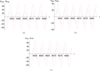 |
Figure 12 Behavior of the system under sinusoidal excitation in the vicinity of the resonant frequency of the tube (V = 1.3 V). Blue: U, red: Q. Top left: normalized experimental time responses. Top right: the numerically determined time responses using the parameters identified from the HBM. Bottom: the temporal responses determined numerically using the parameters identified from the CX-A method. Configuration 1: hm = 0.23 mm, Rm = 5 cm, fm = 45 Hz. (a) Measured time responses. (b) The numerically determined time responses using the parameters identified from the HBM. (c) The numerically determined temporal responses using the parameters identified from the CX-A method. |
For the periodic responses, it is obvious that our identification method is able to reproduce the same regime observed experimentally since we have written the system coordinates in harmonic and periodic forms. Also by using these periodic models, we have been able to identify the parameters of the system that allow to reproduce in the time domain a strongly modulated response very close to the experimentally measured time solution. Thus our simplifying assumption is sufficient for the identification of the parameters in this quasi-periodic regime (the use of a quasi-periodic model to identify our parameters is not necessary).
4.4 Estimated variation of the parameters
In order to analyze the variation of the model parameters as a function of the excitation amplitude, this variation was presented for the three configurations.
The identified parameters of our system are: The forcing term F, the tube eigenpulsation ωt, the tube dissipation λ, the membrane dissipation η, the linear and non-linear membrane stiffness c1 and c3, the coupling coefficient β and the mass term γ. Figures 13–15 show the variations of the parameters as a function of the voltage supplied to the speaker terminal, for the first, second and third configuration respectively. The blue squares correspond to the result given by the HBM and the green triangles by the CX-A method. The beginning and end of the energy pumping are presented by the two grey bands. In the third experiment, we do not see the end of the pumping plateau because our setup cannot reach high enough excitation amplitudes.
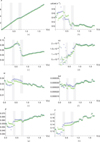 |
Figure 13 The variation of the system parameters as a function of the voltage value sent to the speaker terminal for the first configuration: hm1 = 0.23 mm, Rm1 = 5 cm, fm1 = 45 Hz. The blue squares correspond to the result given by the HBM and the green triangles by the CX-A method. The beginning and the end of the energy pumping are presented by the two grey bands. (a) F as a function of the excitation amplitude. (b) ωt as a function of the excitation amplitude. (c) λ as a function of the excitation amplitude. (d) cη as a function of the excitation amplitude. (e) kl as a function of the excitation amplitude. (f) knl as a function of the excitation amplitude. (g) β as a function of the excitation amplitude. (h) γ as a function of the excitation amplitude. |
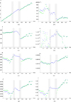 |
Figure 14 The variation of the system parameters as a function of the voltage value sent to the speaker terminal for the second configuration: hm2 = 0.24 mm, Rm2 = 4 cm, fm2 = 44 Hz. The blue squares correspond to the result given by the HBM and the green triangles by the CX-A method. The beginning and the end of the energy pumping are presented by the two grey bands. (a) F as a function of the excitation amplitude. (b) ωt as a function of the excitation amplitude. (c) λ as a function of the excitation amplitude. (d) cη as a function of the excitation amplitude. (e) kl as a function of the excitation amplitude. (f) knl as a function of the excitation amplitude. (g) β as a function of the excitation amplitude. (h) γ as a function of the excitation amplitude. |
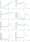 |
Figure 15 The variation of the system parameters as a function of the voltage value sent to the speaker terminal for the third configuration: hm3 = 0.62 mm, Rm3 = 5 cm, fm3 = 45 Hz. The blue squares correspond to the result given by the HBM and the green triangles by the CX-A method. The beginning of the energy pumping is presented by the grey band. (a) F as a function of the excitation amplitude. (b) ωt as a function of the excitation amplitude. (c) λ as a function of the excitation amplitude. (d) cη as a function of the excitation amplitude. (e) kl as a function of the excitation amplitude. (f) knl as a function of the excitation amplitude. (g) β as a function of the excitation amplitude. (h) γ as a function of the excitation amplitude. |
For the second and third configuration, in the pumping area our method encountered a difficulty in identifying the parameters from the CX-A method. The identification for amplitude n + 1 uses as starting values the values identified for amplitude n. In some cases, the optimization routine converges towards obviously nonphysical results for some values of n, but it can converge again towards physical results for greater values of n. We did not display the useless values on the graphs. It happens mostly in the pumping regime, where the responses often deviate from harmonic motion.
Figures 13a, 14a and 15a present the evolution of the forcing term as a function of the excitation amplitude. A linear dependence is observed. This dependence presents an image of the forcing voltage sent to the speaker terminal. The scaled force is defined by :  , where P is the pressure measured inside the loudspeaker coupling box (in Pascal), St and Sm are the cross-sectional areas of the tube and the membrane. From the system equations (1)–(3), we deduce that over the same voltage range, the difference observed in the forcing term for the three configurations is due to the presence of the term
  . Figure 16 presents the superposition of the variation of force scaled by the term
  of the three configurations. In the third experiment, the maximum value of the source voltage is 0.75 V because this level is high enough to observe entirely the pumping plateau. The difference in the variation of the forcing term is related to the difference in the sizes of the membranes in the three configurations.
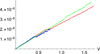 |
Figure 16 Identified normalized force term F (using HBM) divided by the term |

The variation of the natural pulsation of the tube as a function of the voltage sent to the loudspeaker terminal is presented in Figures 13b, 14b and 15b. In these figures one can note the presence of 3 domains of decreasing levels. The first domain is at low excitation amplitude. The second one appears during the energy pumping and the third one in the saturation zone of the membrane. This variation shows that the natural pulsation of the tube is influenced by the operating regime. This small variation can be observed as an effect of the 1:1 resonance capture. It was also noted that the same variation is identified for all three configurations.
The variation of the tube dissipation is the same for all three experiments (Figs. 15, 16c and 15c). An increase of the excitation amplitude leads to an increase of the tube dissipation. It varies from 0.07 for the lowest excitation amplitude to a value of around 0.09 during energy pumping. At saturation, a clear decrease to the value 0.04 is observed. Then at saturation, with the increase of the excitation amplitude, the dissipation, represented by the parameter λ, is slightly increased. This increase does not exceed a value of 0.07 for the first and second experiments in which saturation of the membrane is observed.
The pulsation ωt and the dissipation λ of the tube show the same variation for the three configurations. This shows that our identification method succeeded in reproducing the same results (related to the tube) for the three configurations where we kept the same tube.
Figures 13d, 14d and 15d show the variation of the identified membrane damping term. At low excitation amplitudes the membrane damping term shows large fluctuations. They are very noticeable in the result of the second experiment. These fluctuations may be due to the experimental noise presented at low excitation amplitudes. Since this term is very small, it is may be sensitive to measurement errors. It seems that in this regime, the sensitivity of the model to the damping parameter is small, as the wide range of damping does not change much the amplitudes of the displacement or the velocity.
At low excitation amplitude the dissipation of the membrane is low. When pumping is activated, an increase in dissipation is observed. At saturation, the dissipation of the membrane remains more or less constant.
At low excitation amplitudes, a large amount of energy is dissipated in the tube. With energy pumping, the dissipation introduced by the membrane becomes dominant. At saturation the proportion of energy dissipated in the tube is reduced. This decrease is compensated by the membrane. Then with the increase of the excitation amplitude the part of the energy dissipated by the tube is slightly increased. This can be attributed to the saturation of the membrane, where the vibration amplitude of the membrane reaches its maximum and cannot increase much with increasing excitation amplitude because at these amplitudes the membrane becomes very stiff.
This confirm the fact that our model is able to reproduce the main mechanisms of dissipation composed of three parts. Firstly, at low amplitude most of the energy dissipation of the system is located within the primary linear system while the NES, weakly coupled to the primary system do not participate to dissipation. Secondly, as energy pumping takes place, the dissipation is transferred from the primary system to the NES. Thirdly, during saturation, the two oscillators are strongly coupled and act as a unique oscillator and most of the energy dissipation is achieved by the NES.
The variation of the linear stiffness of the membrane is shown in Figures 13e, 14e and 15e. The linear stiffness shows almost a constant variation outside the pumping region. When the energy pumping was activated, an increase in the value of this term was observed. During energy pumping this stiffness decreases progressively. The linear stiffness of the membrane is equal to  , where
  is the natural frequency of the membrane without taking into account the pre-stress applied to the membrane [4]. This expression explains the difference observed in the stiffness values kl in the three configurations. The linear stiffness depends on the thickness, radius and natural frequency of the membrane, which are not the same in the three configurations.
The non-linear stiffness of the membrane has a constant variation as a function of the excitation amplitude (see Figures 13f, 14f and 15f). The non-linear stiffness of the membrane is equal to  . This shows that the non-linear stiffness depends on the thickness and radius of the membrane.
The variation of the coupling term is presented in Figures 13g, 14g and 15g. An increase in the excitation level is accompanied by an increase in the coupling term. For the three configurations, it could be noticed that the coupling term β remains more or less constant at low amplitude and shows rapid increase of about 20% during energy pumping and saturation. The expression of the coupling term  (see [4]) shows that this term is inversely proportional to the volume of the coupling box. The apparent volume of the coupling box between the membrane and the tube might be reduced by an increase of the inertial effects inside the box then reducing the apparent volume of the coupling box where the pressure effects dominate. Both the high membrane vibration amplitude and the high pressure inside the coupling box impose an apparent elongation of the cm-thick, cylindrical holes connecting the coupling box to the tube and membrane. The mass term follows the variation of the coupling term (see Figs. 13f, 14f and 15f). This term is given by this expression
  . The difference observed between the configurations is due to the change in the size of the membrane. The increase in the apparent membrane mass term could be explained by the low vibration amplitude at low forcing and a strong amplification during energy pumping and saturation, in that case, the membrane drags a larger amount of air in its movement increasing its apparent mass. For example, a latex membrane of 4 cm radius and 0.2 mm thickness weights 1 g and the mass of air that this membrane carries during its movement with a 2 cm amplitude can be roughly estimated at least as that of the volume of a cylinder of diameter equal to that of the membrane and an height of twice the vibrating amplitude corresponding to a volume of air of 0.2l that is a added mass of about 20%, in line with the observed augmentation of the mass term.
Various tests with modifications of the initial parameters gave either the same results for relatively small modifications, or failed convergence for large modifications. It means that the method is rather robust and shows little dispersion, except for cη in the lowest excitation levels as discussed before. We also checked that there was coherence in the relative variation of the parameters. For instance in the firsts tests, when one stiffness parameter had a large value, the others tended to be smaller. The same observation applies to the damping parameters. We also made some checks of parameter independence by fixing some parameters and identifying the other ones. Except for cη there was no situation where two different sets of parameters gave the same responses.
5 Conclusion
In this paper, a method for identifying the parameters of a simplified non-linear model with two degrees of freedom is developed and applied in the vibroacoustic domain. This simplified model represents the behavior of a linear primary acoustic system coupled to a non-linear membrane absorber with a forced harmonic excitation that is valid only within a small frequency–amplitude domain. We calculate the analytic dynamical response of the system, and fit those on experimental data beyond the valid frequency–amplitude domain. To ensure a better agreement with the experiments, we chose to identify a new set of parameters for each excitation amplitude. We calculate the analytic dynamical response with two methods widely used in the non-linear domain: harmonic balance method and complexification-averaging method. These two methods lead to very similar results overall.
We display results for different excitation amplitudes where we observe a linear behavior, a non-linear behavior without energy pumping, energy pumping, and a saturation regime. The method finds parameters for which the model and the experiment are agreeing, over a large frequency–amplitude range. Although the parameters vary only with amplitude, the agreement is good over all the frequency range.
This method gives a better agreement on ridge curves than when the parameters values are obtained from low excitation amplitude experiments, where the nonlinear terms are negligible. The plateau sound level and the pumping activation threshold are at the correct amplitudes.
We compare experimental data and the time integration of the initial model, with the identified parameters. The same regimes are observed, including the quasi-periodic regime, even if the parameter values are identified as periodic analytic responses.
The variation of the system parameters as a function of the excitation amplitude is almost the same for both methods, which can be seen as a cross validation. The identified parameters have physically acceptable magnitudes and the observed variations are compatible with the physical phenomenons. The method is successfully applied on two other sets of experiments where the membrane characteristics are modified.
Despite the fact that the complexification-averaging method is usable for the analysis of highly modulated responses, it is less robust than the harmonic balance method in the energy pumping zone, when the frequency response of the system shows strong fluctuations. As identification by harmonic balance method is faster than the complexification-averaging method, it therefore seems preferable to use the harmonic balance method for identification.
Conflict of interest
The author declare no conflict of interest.
References
- O. Gendelman, L.I. Manevitch, A.F. Vakakis, R. M’Closkey: Energy pumping in nonlinear mechanical oscillators: Part I – dynamics of the underlying hamiltonian systems. Journal of Applied Mechanics 68, 1 (2000) 34–41. https://doi.org/10.1115/1.1345524. [Google Scholar]
- A.F. Vakakis, O. Gendelman: Energy pumping in nonlinear mechanical oscillators: Part II – resonance capture. Journal of Applied Mechanics 68, 1 (2000) 42–48. https://doi.org/10.1115/1.1345525. [Google Scholar]
- B. Cochelin, P. Herzog, P.-O. Mattei: Experimental study of targeted energy transfer from an acoustic system to a nonlinear membrane absorber, Comptes Rendus Mécanique 334, 11 (2006) 639–644. https://doi.org/10.1016/j.crme.2006.08.005. [CrossRef] [Google Scholar]
- R. Bellet, B. Cochelin, P. Herzog, P.-O. Mattei: Experimental study of targeted energy transfer from an acoustic system to a nonlinear membrane absorber. Journal of Sound and Vibration 329, 14 (2010) 2768–2791. https://doi.org/10.1016/j.jsv.2010.01.029. [CrossRef] [Google Scholar]
- R. Mariani, S. Bellizi, B. Cochelin, P. Herzog, P.-O. Mattei: Toward an adjustable nonlinear low frequency acoustic absorber. Journal of Sound and Vibration 330, 22 (2011) 5245–5258. https://doi.org/10.1016/j.jsv.2011.03.034. [CrossRef] [Google Scholar]
- R. Bellet, B. Cochelin, R. Côte, P.-O. Mattei: Enhancing the dynamic range of targeted energy transfer in acoustics using several nonlinear membrane absorbers. Journal of Sound and Vibration 331, 26 (2012) 5657–5668. https://doi.org/10.1016/j.jsv.2012.07.013. [CrossRef] [Google Scholar]
- J. Shao, B. Cochelin: Theoretical and numerical study of targeted energy transfer inside an acoustic cavity by a non-linear membrane absorber. International Journal of Non-Linear Mechanics 64 (2014) 85–92. https://doi.org/10.1016/j.ijnonlinmec.2014.04.008. [CrossRef] [Google Scholar]
- J. Shao, T. Zeng, X. Wu: Study of a nonlinear membrane absorber applied to 3d acoustic cavity for low frequency broadband noise control. Materials (Basel) 12, 7 (2019) 1138. https://doi.org/10.3390/ma12071138. [CrossRef] [PubMed] [Google Scholar]
- J. Shao, Q. Luo, G. Deng, T. Zeng, J. Yang, X. Wu, C. Jin: Experimental study on influence of wall acoustic materials of 3d cavity for targeted energy transfer of a nonlinear membrane absorber, Applied Acoustics 184 (2021) 108342. https://doi.org/10.1016/j.apacoust.2021.108342. [CrossRef] [Google Scholar]
- L.J. Sivian: Acoustic impededance of small orifices. The Journal of the Acoustical Society of America 7 (1935) 94–101. https://doi.org/10.1121/1.1915795. [CrossRef] [Google Scholar]
- R.H. Bolt, S. Labate, U. Ingard: The acoustic reactance of small circular orifices. The Journal of the Acoustical Society of America 21, 2 (1949) 94–97. https://doi.org/10.1121/1.1906488. [CrossRef] [Google Scholar]
- V. Alamo Vargas, E. Gourdon, A. Ture Savadkoohi: Nonlinear softening, hardening behavior in helmholtz resonators for nonlinear regimes. Nonlinear Dynamics 91 (2018) 217–231. https://doi.org/10.1007/s11071-017-3864-8. [CrossRef] [Google Scholar]
- E. Gourdon, A. Ture Savadkoohi, V. Alamo Vargas: Targeted energy transfer from one acoustical mode to an helmholtz resonator with nonlinear behavior. Journal of Vibration and Acoustics 140, 6 (2018) 061005. https://doi.org/10.1115/1.4039960. [CrossRef] [Google Scholar]
- T.D. Burton, On the amplitude decay of strongly non-linear damped oscillators. Journal of Sound and Vibration 87, 4 (1983) 535–541. https://doi.org/10.1016/0022-460X(83)90504-7. [CrossRef] [Google Scholar]
- S. Wang, B. Tang: Estimating quadratic and cubic stiffness nonlinearity of a nonlinear vibration absorber with geometric imperfections. Measurement 185 (2021) 110005. https://doi.org/10.1016/j.measurement.2021.110005. [CrossRef] [Google Scholar]
- G. Kenderi, A. Fidlin: Nonparametric identification of nonlinear dynamic systems using a synchronisation-based method. Journal of Sound and Vibration 333, 24 (2014) 6405–6423. https://doi.org/10.1016/j.jsv.2014.07.021. [CrossRef] [Google Scholar]
- H.V.H. Ayala, L. dos Santos Coelho: Cascaded algorithm for nonlinear system identification based on correlation functions and radial basis functions neural networks. Mechanical Systems and Signal Processing 68–69 (2016) 378–393. https://doi.org/10.1016/j.ymssp.2015.05.022. [CrossRef] [Google Scholar]
- A. Lund, S.J. Dyke, W. Song, I. Bilionis: Identification of an experimental nonlinear energy sink device using the unscented kalman filter. Mechanical Systems and Signal Processing 136 (2020) 106512. https://doi.org/10.1016/j.ymssp.2019.106512. [CrossRef] [Google Scholar]
- A.H. Nayfeh: Perturbation Methods, Wiley, New York, 1973. [Google Scholar]
- A.H. Nayfeh, D.T. Mook: Nonlinear Oscillations, Wiley, New York, 1979. [Google Scholar]
- R.E. Mickens: Oscillations in Planar Dynamic Systems, World Scientific. https://doi.org/10.1142/2778. [Google Scholar]
- L.I. Manevitch: The description of localized normal modes in a chain of nonlinear coupled oscillators using complex variables. Nonlinear Dynamics 25 (2001) 95–109. https://doi.org/10.1023/A:1012994430793. [CrossRef] [Google Scholar]
- Wolfram Research, Inc.: Mathematica, Version 13, Champaign, IL, 2022. https://www.wolfram.com/mathematica. [Google Scholar]
Cite this article as: Bouzid I. Côte R. Fakhfakh T. Haddar M. & Mattei P-O. 2022. Identification of the parameters of a simplified 2 degree of freedom model of a nonlinear vibroacoustic absorber coupled to an acoustic system in linear and nonlinear forced regimes. Acta Acustica, 6, 60.
All Figures
|
Figure 1 Experimental fixture. |
| In the text | |
|
Figure 2 schematic diagram of the experimental set-up and equivelent mechanical representation. |
| In the text | |
|
Figure 3 Experimentally determined amplitude-frequency response surfaces of the tube (a) and membrane (b) for configuration 1: hm = 0.23 mm, Rm = 5 cm, fm = 45 Hz. |
| In the text | |
|
Figure 4 Normalized frequency responses of the membrane determined analyticly (red) and experimentally (blue). (a) maximum analytic solution (b) minimum analytic solution. |
| In the text | |
|
Figure 5 Normalized results of identification (V = 0.01 V). Blue: identification using HBM. Green: CX-A method. Red: experimental frequency response functions. (a) tube displacement, (b) membrane displacement. Configuration 1: hm = 0.23 mm, Rm = 5 cm, fm = 45 Hz. |
| In the text | |
|
Figure 6 Normalized results of identification (V = 0.27 V). Blue: identification using HBM. Green: CX-A method. Red: experimental frequency response functions. Gray dots: discontinuity, guide to the eye. (a) tube displacement, (b) membrane displacement. Configuration 1: hm = 0.23 mm, Rm = 5 cm, fm = 45 Hz. |
| In the text | |
|
Figure 7 Normalized results of identification (V = 0.52 V). Blue: identification using HBM. Green: CX-A method. Red: experimental frequency response functions. Gray dots: discontinuity, guide to the eye. (a) tube displacement, (b) membrane displacement. Configuration 1: hm = 0.23 mm, Rm = 5 cm, fm = 45 Hz. |
| In the text | |
|
Figure 8 Normalized results of identification (V = 1.12 V). Blue: identification using HBM. Green: CX-A method. Red: experimental frequency response functions. Gray dots: discontinuity, guide to the eye. (a) tube displacement, (b) membrane displacement. Configuration 1: hm = 0.23 mm, Rm = 5 cm, fm = 45 Hz. |
| In the text | |
|
Figure 9 Ridge curves of U (maximum amplitudes over all frequency range). Red: normalized experimental data. Blue: numerical integration of the equations with parameters identified by HBM. Green: numerical integration with parameters identified by CX-A. Continuous black: numerical integration with parameters determined experimentally at low excitation amplitude. Dashed black: numerical intergration with the mean parameters determined by HBM inside the pumping zone. Configuration 1: hm = 0.23 mm, Rm = 5 cm, fm = 45 Hz. |
| In the text | |
|
Figure 10 Time series of the two degrees of freedom of the system. f = 85 Hz, V = 0.025 V. The blue curves show the scaled displacement of the air at the end of the tube and the red curves show the scaled displacement at the center of the membrane. Top left: measured time responses. Top right: the numerically determined time responses using the parameters identified from the HBM. Bottom: the temporal responses determined numerically using the parameters identified from the CX-A method. Configuration 1: hm = 0.23 mm, Rm = 5 cm, fm = 45 Hz. (a) The measured time responses. (b) The numerically determined time responses using the parameters identified from the HBM. (c) The numerically determined time responses using the parameters identified from the CX-A method. |
| In the text | |
|
Figure 11 Time series of the two degrees of freedom of the system. f = 85 Hz, V = 0.61 V. The blue curves show the scaled displacement of the air at the end of the tube and the red curves show the scaled displacement at the centre of the membrane. Top left: measured time responses. Top right: the numerically determined time responses using the parameters identified from the HBM. Bottom: the temporal responses determined numerically using the parameters identified from the CX-A method. Configuration 1: hm = 0.23 mm, Rm = 5 cm, fm = 45 Hz. (a) Measured time responses. (b) The numerically determined time responses using the parameters identified from the HBM. (c) The numerically determined temporal responses using the parameters identified from the CX-A method. |
| In the text | |
|
Figure 12 Behavior of the system under sinusoidal excitation in the vicinity of the resonant frequency of the tube (V = 1.3 V). Blue: U, red: Q. Top left: normalized experimental time responses. Top right: the numerically determined time responses using the parameters identified from the HBM. Bottom: the temporal responses determined numerically using the parameters identified from the CX-A method. Configuration 1: hm = 0.23 mm, Rm = 5 cm, fm = 45 Hz. (a) Measured time responses. (b) The numerically determined time responses using the parameters identified from the HBM. (c) The numerically determined temporal responses using the parameters identified from the CX-A method. |
| In the text | |
|
Figure 13 The variation of the system parameters as a function of the voltage value sent to the speaker terminal for the first configuration: hm1 = 0.23 mm, Rm1 = 5 cm, fm1 = 45 Hz. The blue squares correspond to the result given by the HBM and the green triangles by the CX-A method. The beginning and the end of the energy pumping are presented by the two grey bands. (a) F as a function of the excitation amplitude. (b) ωt as a function of the excitation amplitude. (c) λ as a function of the excitation amplitude. (d) cη as a function of the excitation amplitude. (e) kl as a function of the excitation amplitude. (f) knl as a function of the excitation amplitude. (g) β as a function of the excitation amplitude. (h) γ as a function of the excitation amplitude. |
| In the text | |
|
Figure 14 The variation of the system parameters as a function of the voltage value sent to the speaker terminal for the second configuration: hm2 = 0.24 mm, Rm2 = 4 cm, fm2 = 44 Hz. The blue squares correspond to the result given by the HBM and the green triangles by the CX-A method. The beginning and the end of the energy pumping are presented by the two grey bands. (a) F as a function of the excitation amplitude. (b) ωt as a function of the excitation amplitude. (c) λ as a function of the excitation amplitude. (d) cη as a function of the excitation amplitude. (e) kl as a function of the excitation amplitude. (f) knl as a function of the excitation amplitude. (g) β as a function of the excitation amplitude. (h) γ as a function of the excitation amplitude. |
| In the text | |
|
Figure 15 The variation of the system parameters as a function of the voltage value sent to the speaker terminal for the third configuration: hm3 = 0.62 mm, Rm3 = 5 cm, fm3 = 45 Hz. The blue squares correspond to the result given by the HBM and the green triangles by the CX-A method. The beginning of the energy pumping is presented by the grey band. (a) F as a function of the excitation amplitude. (b) ωt as a function of the excitation amplitude. (c) λ as a function of the excitation amplitude. (d) cη as a function of the excitation amplitude. (e) kl as a function of the excitation amplitude. (f) knl as a function of the excitation amplitude. (g) β as a function of the excitation amplitude. (h) γ as a function of the excitation amplitude. |
| In the text | |
|
Figure 16 Identified normalized force term F (using HBM) divided by the term |
| In the text | |
Current usage metrics show cumulative count of Article Views (full-text article views including HTML views, PDF and ePub downloads, according to the available data) and Abstracts Views on Vision4Press platform.
Data correspond to usage on the plateform after 2015. The current usage metrics is available 48-96 hours after online publication and is updated daily on week days.
Initial download of the metrics may take a while.