| Issue |
Acta Acust.
Volume 9, 2025
|
|
|---|---|---|
| Article Number | 53 | |
| Number of page(s) | 16 | |
| Section | Environmental Noise | |
| DOI | https://doi.org/10.1051/aacus/2025034 | |
| Published online | 19 August 2025 | |
Scientific Article
Spatial attenuation characteristics and influencing factors of traffic noise in high-density cities: A case study of Tianjin, China
1
School of Architecture and Art Design Hebei University of Technology, Tianjin, 300130, China
2
Hebei Key Laboratory of Healthy Human Settlements, Tianjin, 300130, China
3
Tianjin Municipal Engineering Design & Research Institute Co., Ltd., Tianjin, 300392, China
4
School of Science Hebei University of Technology, Tianjin, 300401, China
5
Institute for Environmental Design and Engineering, The Bartlett, University College London, London, WC1H 0NN, United Kingdom
* Corresponding author: This email address is being protected from spambots. You need JavaScript enabled to view it.
Received:
14
November
2024
Accepted:
11
July
2025
Abstract
Amid increasing concerns regarding traffic noise pollution, existing research has demonstrated correlations between spatial noise distribution and urban parameters including land use patterns, traffic flow dynamics, and building layouts. Nevertheless, critical gaps persist in establishing actionable frameworks to identify and mitigate high-noise pollution zones during urban planning processes, particularly in high-density cities. This study systematically identifies the spatial attenuation characteristics and determinants of traffic noise in Tianjin through noise map, clustering analysis, correlation analysis, structural equation modelling. The findings revealed that (1) the units with traffic noise spatial attenuation can be classified into four types: attenuation primarily in high noise areas, attenuation primarily in medium noise areas, attenuation primarily in low noise areas, and low total attenuation. (2) The attenuation values of noise in the high and medium noise areas are positively correlated with the ground space index, building boundary density, architectural landscape shape index, and proportion of residential land, and are negatively correlated with the proportion of green space. (3) Through structural equation modelling analysis, this study revealed that the building indicators have a greater effect on the attenuation values of noise in the medium noise areas; the road indicators have a greater effect on the attenuation values of noise in the high noise areas; and the land use indicators have greater effects on high, medium and low noise areas. This study provides evidence-based urban planning strategies for mitigating traffic noise exposure in high-density cities.
Key words: Traffic noise / noise map / high-density cities
© The Author(s), Published by EDP Sciences, 2025
 This is an Open Access article distributed under the terms of the Creative Commons Attribution License (https://creativecommons.org/licenses/by/4.0), which permits unrestricted use, distribution, and reproduction in any medium, provided the original work is properly cited.
1. Introduction
Among the 7.5 billion people worldwide, 55% are living in cities, which, according to data from the United Nations, will increase to two-thirds by 2050 [1]. With the continuous increase in urban size and density, noise pollution in cities is becoming increasingly serious. A noisy environment can interfere with the daily life of urban residents and cause health problems such as sleep disorders and mental stress [2–5]. The main component of urban noise is traffic noise [6]. It refers to the sound that hinders people’s normal life and work when vehicles are running. The main factors affecting the spatial distribution of traffic noise levels include land use, traffic organisation, architectural forms along streets, greening along streets, etc [7–10].
According to relevant studies, land use is an important factor that affects the spatial distribution of traffic noise. Yuan researched the relationships between three factors, namely, land coverage, land use, and urban form, and noise levels in the central urban area of Wuhan and reported that the proportions of commercial land, industrial land, and residential land had positive effects on noise levels [11]. By studying the factors affecting the noise level in Greater London, Xie reported that residential land was significantly negatively correlated with the noise level and that the proportions of non-residential land and land used for roads were significantly positively correlated with the noise level [12].
With respect to the effect of traffic organisation on the spatial distribution of traffic noise, Salomons used Amsterdam and Rotterdam in Holland as the objects of study to analyse the relationships between urban traffic factors and the spatial distribution of traffic noise and reported that the average level of noise increased with increasing density of the road network and the number of 24 h driving kilometres per square kilometre [13]. Ryu studied the relationship between urban traffic factors and traffic noise levels in Cheongju, South Korea, by building a spatial statistical model and reported that the traffic volume, vehicle speed, and road area density positively influence the road traffic noise level [14].
In terms of the effect of the building layout on the spatial distribution of traffic noise, Han studied the effect of urban building layout on traffic noise in the Shenzhen metropolitan area of China through multisource data such as noise monitoring data, remote sensing data, and geographic information data [15]. The scattered distribution and irregular shape of buildings were beneficial to the attenuation of regional environmental noise, and the continuity of buildings along the streets can effectively alleviate the effects of traffic noise. Wu used the actual streets of high-density cities as the objects of study to analyse the relationship between urban street spatial parameters and sound propagation and reported that the attenuation of traffic noise decreased with increasing cross-sectional and planar enclosures of roads [16]. Zhou et al. (2024) studied the relationship between building layout indicators and traffic noise distribution, and reported that the building density, floor space index, building boundary density, and architectural landscape shape index were significantly negatively correlated with the noise level (L70∼L90) in low noise areas [17]. In addition, many studies have investigated the effects of meteorological conditions, landscape greening, road sections, etc., on traffic noise attenuation, which provides useful guidance for improving the urban traffic noise environment [18–20].
Traffic noise originates from the road and dissipates in space, following the attenuation law of noise level, which divides it into high, medium, and low noise areas. Cities are organisms that have developed over many years. Units with the same land use type have similar spatial organizational structures, which in turn leads to similar spatial distribution characteristics of traffic noise [9, 21]. Clustering methods can be used to classify units with similar noise spatial distributions.
With the development of geographic information technology and noise mapping technology, large-scale and low-cost simulation of urban spatial noise distribution has become possible [22, 23]. However, performing large-scale and repeated simulations of traffic noise spatial distribution remains a significant challenge in the context of urban planning. Rapidly identifying and reducing the area of high noise area through spatial morphological indicators is an effective way to reduce the impact of traffic noise.
To rapidly identify high-noise areas in cities, this paper builds on previous studies [14, 16] and focuses on the following issues: (1) determining the types of noise attenuation in high-density cities; (2) identifying the main influencing factors in high, medium, and low noise attenuation zones; and (3) exploring the impact pathways of noise attenuation across these zones. To address these questions, Tianjin was selected as the study area. Firstly typical regional noise maps were generated, and clustering methods were applied to determine the types and characteristics of spatial attenuation of traffic noise in different types of land use units; secondly, correlation analysis was used to determine the relationship between urban spatial element indicators and noise attenuation values in different noise areas; finally, a structural equation model was used to explore the impact path and weight of urban spatial elements on the spatial attenuation of noise in different noise areas.
2. Methods
2.1. Study area
A high-density city is a compact and intensive city centred on population agglomeration and accompanied by high-density compound development of multiple factors, including land use, economy, transportation, etc [24]. Tianjin has a permanent population of 13.73 million and an urban built-up area of approximately 1237 square kilometres, making it a typical high-density city. As shown in Figure 1, the study area is in downtown Tianjin, covering an area of 125 square kilometres, including the entire area of Heping District and Hongqiao District; most of the areas of Hebei District and Nankai District (> 50%); and parts of Hexi District, Hedong District, Beichen District, Xiqing District and Dongli District (< 50%). This area is the central area of Tianjin for political, cultural, and economic activities, covering urban functions such as residences, commerce, education, scientific research, and green space. This study divided the area into five hundred 500 * 500 m research units, which can provide sufficient samples for analysing the relationship between the urban spatial form and traffic noise attenuation [25–28].
 |
Figure 1. Study area and location. |
2.2. Production of the noise map and selection of the noise spatial attenuation indicators
(1) Production of the noise map
The traffic noise map was produced via CadnaA with the CNOSSOS-EU standard, the most widely used standard in Europe. Studies have shown that, compared with the previously used CRTN-TRL method, the CNOSSOS-EU method can more accurately reflect the actual situation of road traffic noise [29, 30]. In accordance with the strategic noise mapping requirements of 2002/49/EC [31], a noise map was drawn at a height of 4 m above the ground, with a distance of 10 m between the calculated grids. The average absorption coefficient of the building, α, equals 0.4 [32]. This study focused on hard ground, with the overall ground coefficient G set to 0.2 [33].
Following the generation of noise maps, eight strategically selected monitoring points within the Fengmao Li neighborhood (Hongqiao District, Tianjin) were established for empirical validation through on-site noise level measurements, with spatial distribution detailed in Figure 2. In accordance with acoustic propagation principles, monitoring points were strategically positioned along arterial/collector roads and at intra-block sampling nodes representing characteristic urban morphologies. The measurements were taken during the peaktraffic period on weekdays from 7:00 to 9:00 AM, with each measurement lasting 10 min. During the measurement, the sound level meter was positioned 1.5 m above the ground and at least 3.5 m away from reflective surfaces. An AWA5688 model sound level meter was used, with an accuracy class of Type 2. Prior to measurements, the sound level meter was calibrated using an HS6020 model sound calibrator.
 |
Figure 2. Distribution of noise measurement points. |
Following field measurements, a comparative analysis between empirically acquired data and noise mapping outputs (Fig. 3) revealed a mean discrepancy of 2.2 dB(A) between observed and simulated values, demonstrating sufficient accuracy for urban-scale noise modelling applications [34].
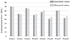 |
Figure 3. Comparison of the simulated noise values at each point with the measured values. |
(2) Selection of the noise spatial attenuation indicators
To analyse the spatial distribution characteristics of traffic noise in detail, this study employed the spatial statistics noise level (L n) as the observation indicator, in which L n represents the value that n% of the noise level within the statistical unit exceeds, for example, L 33 represents the value that 33% of the noise level in the unit exceeds, and L 73 represents the value that 73% of the noise level in the area exceeds [9, 25]. This indicator can reflect the spatial distribution of noise.
To determine the attenuation intervals of high-density urban traffic noise, this study applied the K-means clustering algorithm to group the statistical percentile noise values of each spatial unit. The optimal number of classification intervals was determined to be three, based on a comprehensive analysis using both the elbow rule and contour coefficient method [35–37]. Each research unit was divided into three noise areas: the high noise area, the medium noise area and the low noise area, which fell into Lmax to L33, L34 to L72, and L73 to Lmin, respectively. As shown in Figure 4, according to the division of the noise areas, this study uses Lmax − 33, L34 − 72, and L73 − min to represent the attenuation values of noise in the high, medium, and low noise areas, respectively.
 |
Figure 4. Noise attenuation range and attenuation value diagram. |
2.3. Selection of the urban spatial form indicators
This study primarily analysed the effect of the urban building layout, road organisation, and land use on the spatial attenuation of traffic noise. The building layout indicators included the average building height (ABH), ground space index (GSI), floor space index (FSI), building boundary density (BBD), and architectural landscape shape index (ALSI). The road organisation indicators included the road length index (RLI), road area density (RAD), road landscape shape index (RLSI), and trunk road length index (TRLI). The land use indicators included the proportion of commercial land (PC), proportion of residential land (PA), proportion of traffic land (PT), proportion of green space (PG), degree of land mix (DLM), and degree of functional mixing (DFM) [12, 38–40]. See Appendix A for the calculation methods of the indicators. The building data and points of interest (POI)were from the Amap open platform, and the road organisation and land use attribute data were from Tianjin Urban Planning and Design Institute Co., Ltd. The descriptive statistics of the various indicators are shown in Table 1.
Descriptive statistics of urban space indicators.
2.4. Data analysis
(1) K-Means clustering
The K-means clustering is a distance-based clustering algorithm, the core idea is to group similar samples into the same subset based on similarity measures, such that the variance within each subset is minimized, while the variance between different subsets is maximized [41]. To determine the spatial attenuation characteristics of traffic noise in high-density cities, this study first calculated the spatial statistical noise value (Ln) of each unit, and calculated the values of Lmax − 33, L34 − 72, and L73 − min for each unit. According to the numerical distributions of Lmax − 33, L34 − 72, and L73 − min of each unit and by using the K-means clustering method, as shown in Figure 5, the best clustering number was determined to be 4 based on the elbow rule and contour coefficient method, that is, the units in the research range can be classified into four types of noise attenuation. The procedure was performed via Sci-kit learn 1.1.2 in a Python 3.8.5 environment.
 |
Figure 5. Noise attenuation classification using the Elbow Rule and Silhouette Coefficient method. (a) The elbow rule was used to determine the optimal number of clusters for the type of unit noise attenuation. (b) The silhouette coefficient values were used to determine the optimal number of clusters for the cell noise attenuation type. |
(2) Correlation analysis
This study used Pearson correlation analysis to measure the relationship between the urban spatial form indicators and spatial attenuation values of traffic noise. The process was carried out via SPSS (version 26), and correlation analysis was carried out among the high, medium, and low noise areas and 15 urban spatial form indicators.
(3) Principal component analysis
In the analysis of the effect path, too many indicators lead to too many paths, which not only increases the difficulty of the calculation but also makes it difficult to systematically reflect the comprehensive effects of various indicators. To reduce the indicator dimensions in the path analysis and analyse the comprehensive effects of various indicators on noise, the dimensions of the three indicators, namely, the building layout, road organisation and land use, were reduced through principal component analysis (PCA). The statistical analyses were conducted with SPSS (version 26).
(4) Structural equation path analysis
To clarify the effect of urban spatial form indicators on the spatial attenuation of traffic noise and measure the degree of effect on each path, this study adopted the structural equation modelling (SEM) to construct a path analysis model. Structural equation modelling embodies a theory-driven methodology that integrates theoretical frameworks with empirical data analysis, enabling systematic examination of hypothesized causal pathways among observed variables and latent constructs specified a priori [42].
The model should set the unilateral effect among the indicators in advance and then obtain the direct and indirect acting coefficients among the indicators. The analysis process was performed via SPSS (version 24).
 |
Figure 6. The numerical distribution of each attenuation interval in the four noise spatial attenuation types. |
3. Results
3.1. Spatial attenuation and spatial characteristics of traffic noise
(1) Types of spatial attenuation of noise
Figure 6 shows the distribution of the noise spatial attenuation values (Lmax − 33, L34 − 72, and L73 − min) of the four types of noise attenuation units clustered via theK-means method. As shown in the figure, for the unit in Figure 6a, the mean value of Lmax − 33 was the largest, which was 15.5 dBA, with attenuation occurring primarily in high noise areas. For the unit in Figure 6b, the mean value of L34 − 72 was the largest, exceeding 12.2 dBA, with attenuation primarily in medium noise areas; for the unit in Figure 6c, the mean value of L73 − min was the largest, exceeding 17.5 dBA, with attenuation primarily in low noise areas; for the unit in Figure 6d, the mean values of both Lmax − 33, L34 − 72, and L73 − min were lower than 10 dBA, which belong to the low total attenuation types.
(2) Spatial distribution characteristics of the four types of noise units
Figure 7 shows the spatial distribution of the four types of noise spatial attenuation units. As shown in the figure, there were 111 units with attenuation primarily in high noise areas, indicating poor spatial agglomeration without an obvious law of distribution. There were 166 units with attenuation primarily in medium noise areas, showing higher spatial agglomeration and greater distribution more in the middle of the study area. There were 167 units with attenuation primarily in low noise areas, showing the strongest spatial agglomeration and primary distribution in the surrounding areas of water systems, including the Haihe River and South Canal. There were 56 units with low total attenuation, showing the worst spatial agglomeration and primary distribution along the river and in park areas.
 |
Figure 7. Spatial distribution of the four noise spatial attenuation types in the study area. |
(3) Spatial factor characteristics of the four types of noise units
Figure 8 shows the standardised mean values of the indicators corresponding to the four types of units. The dashed line in the figure has a scale of 0, which also represents the standardised mean values of the indicators of all the research units. As shown in the figure, the units with attenuation, primarily in high noise areas (Fig. 8a), were mainly residential lands where the average building height was slightly lower than the mean value of all the units; the ground space index, building boundary density, and architectural landscape shape index were relatively high; and the road organisation indicators were all lower than the mean value of all the units. The units with attenuation, primarily in medium noise areas (Fig. 8b), represented a high proportion of residential land and a low proportion of green spaces. Except for the average building height, all the values of the building layout indicators were greater than the mean value of all the units, and the road organisation indicators were slightly greater than the mean value. The units with attenuation, primarily in low noise areas (Fig. 8c), represented a high proportion of public service facilities, traffic land, and green spaces. Except for the average building height, all the values of the building layout indicators were lower than the mean value of all the units, and the road organisation indicators were higher than the mean value of all the units. The units with low total attenuation (Fig. 8d) presented much lower values of most indicators than the mean value of all the units, except for the proportion of green spaces, which was much greater than that of all the units.
 |
Figure 8. Radar charts of standardized numerical characteristics of indicators corresponding to each type of attenuation: (a) high-value attenuation type; (b) medium-value attenuation type; (c) low-value attenuation type; (d) low total attenuation type. |
3.2. Relationship between urban spatial factors and noise spatial attenuation
To analyse the relationship between urban spatial factors and the spatial attenuation of traffic noise, this study conducted a correlation analysis between 15 urban factors in each unit and the noise levels of Lmax − 33, L34 − 72, and L73 − min. As shown in Figure 9, except for the average building height and floor space index, other building layout indicators (ground space index, building boundary density, and architectural landscape shape index) were significantly positively correlated with Lmax − 33. The road organisation indicators (road length index, road area density, road landscape shape index, and trunk road length index) were significantly negatively correlated with Lmax − 33. Among the land use indicators, except for the proportion of residential land and degree of functional mixing, other indicators (proportion of commercial land, proportion of traffic land, proportion of green space and degree of land mix) were significantly negatively correlated with Lmax − 33.
 |
Figure 9. Correlation analysis between urban spatial elements and spatial attenuation index of traffic noise. |
The analysis results indicated that, except for the average building height, other building layout indicators (ground space index, floor space index, building boundary density, and architectural landscape shape index) were significantly positively correlated with L34 − 72. Except for the road landscape shape index, other road organisation indicators (road length index, road area density, and trunk road length index) were significantly positively correlated with L34 − 72. The proportion of residential land and degree of functional mixing were significantly positively correlated with L34 − 72, whereas the proportion of green space was significantly negatively correlated with L34 − 72.
The analysis results revealed that, except for the average building height, other building layout indicators (ground space index, floor space index, building boundary density, architectural landscape shape index, and proportion of residential land) were significantly negatively correlated with L73 − min. The road organisation indicators (road length index, road area density, road landscape shape index, and trunk road length index) were significantly positively correlated with L73 − min. The proportion of residential land was significantly negatively correlated with L73 − min, whereas the proportion of commercial land, proportion of traffic land, degree of land mix, and degree of functional mixing were significantly positively correlated with L73 − min.
3.3. Paths of urban spatial factors affecting the spatial attenuation of traffic noise
To clarify the paths affecting urban spatial form indicators of traffic noise spatial attenuation and measure the effect of each path, this study adopted the structural equation method to construct a path analysis model [43, 44]. The path analysis model was built on the basis of the following hypotheses.
-
(1)
Land use affects road network organisation;
-
(2)
Land use affects the building layout;
-
(3)
There is a mutual effect between building layout and road organisation;
-
(4)
All the urban spatial form indicators affect the three noise spatial attenuation indicators; and
-
(5)
The noise attenuation values in high noise areas affected those in medium and low noise areas, and the noise attenuation values in medium noise areas affected those in low noise areas.
On the basis of the above hypotheses, the paths affecting the indicators were graphically illustrated to obtain the hypothesis meta-model (Fig. 10), which was used for building the initial path analysis model of traffic noise attenuation (Fig. 11). To reduce the dimension of analysis, the dimensionality of the factors building layout, road organisation and land use was reduced. After standardisation of the indicators, determination of the number of principal components on the basis of theeigenvalues and variance explainability, and construction of the common factor expression, six principal components were extracted from 15 urban spatial indicators to analyse the affecting paths.
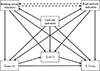 |
Figure 10. Meta model of “Influencing factors-traffic noise attenuation”. |
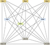 |
Figure 11. Initial model of “Influencing factors-traffic noise attenuation”. |
Among the six principal components, two principal components, PCB1 and PCB2, explained 92.5% of the building layout indicators (PCB1: 60.6% and PCB2: 31.9%); PCR, as the only principal component of the road organisation indicators, explained 84.5% of the road organisation indicators; and three principal components, PCL1, PCL2, and PCL3, explained 80.8% of the land use indicators (PCL1: 32.4%, PCL2: 28.3%, and PCL3: 20.1%).
The variance percentage and factor loading of each principal component are shown in Table 2. PCB1 mainly explained the changes in the building boundary density (30.4%), ground space index (29.4%) and architectural landscape shape index (26.0%), whereas PCB2 mainly explained the changes in the average building height (57.6%) and floor space index (32.6%). PCR had similar explanations for the road length index (38.3%), road area density (29.0%) and road landscape shape index (32.7%). PCL1 mainly explained the changes in the proportion of residential land (57.6%) and the proportion of green space (23.3%). PCL2 mainly explained the changes in the degree of functional mixing (34.5%), degree of land mixing (25.0%) and proportion of green space (23.4%). PCL3 mainly explained the changes in the proportion of commercial land (53.0%) and degree of land mixing (20.7%).
Contribution rate and loading of each principal component variable.
This study adopted the chi-square divided by the degrees of freedom (χ 2/df), GFI, AGFI, AIC, BIC and other output parameters as the evaluation criteria to modify the initial path analysis model by deleting the nonsignificant paths with P > 0.05 in the model fit and reevaluating the goodness-of-fit of the model [45, 46]. The final AIC, BIC and CAIC values all decreased significantly, indicating that the goodness-of-fit of the model gradually increased. The other output parameters are shown in Table 3.
Path analysis model parameter tuning intervals and tuning results.
Figure 12 presents the modified model, which shows the effects of land use on buildings and roads and the direct and indirect effects of the three indicators on different noise attenuation indicators. The black arrows indicate significant factors associated with positive effects of response variables, the red arrows indicate those associated with negative effects, the arrow widths correspond to the absolute values of the relative effects, and only significant predictors are shown in the figure.
 |
Figure 12. Modified model of “Influencing factors-traffic noise attenuation”. |
Tables 3, 4, and 5 show the coefficients of the direct, indirect and total effects of each principal component on Lmax − 33, L34 − 72, and L73 − min, respectively. We eliminated the indirect path with a coefficient absolute value less than 0.05. Table 4 presents the effect of each principal component on Lmax − 33. PCR has the maximum direct effect on Lmax − 33, with a coefficient of −0.324, indicating that road organisation factors have crucial effects on the high-value attenuation of traffic noise. The coefficient of the direct effect of PCL1 on Lmax − 33 is −0.302. PCL2 and PCL3 indirectly affected Lmax − 33 by affecting PCR, with coefficients of −0.115 and −0.073, respectively. The results revealed that land use factors directly affected Lmax − 33; furthermore, they also had indirect effects on Lmax − 33 by affecting road organisation.
Summary of direct and indirect effects of each principal component factor on L max − 33.
Summary of direct and indirect effects of each principal component factor on L 34 − 72.
Summary of direct and indirect effects of each principal component factor on L 73 − min.
Table 5 presents the effect of each principal component on L34 − 72. PCB1 had the maximum direct effect on L34 − 72, with a coefficient of 0.517. The analysis of the contribution of each indicator to PCB1 showed that GSI, BBD and BLSI contributed greatly to PCB1 (Tab. 1). The coefficient of the total effect of PCL1 on L34 − 72 was −0.467, where the coefficient of the direct effect was −0.249, and the coefficient of the indirect effect on L34 − 72 by affecting PCB1 was −0.268. PCL2 and PCL3 had indirect effects on L34 − 72 by affecting PCB1, with coefficients of 0.259 and −0.068, respectively. These results showed that land use factors directly affect L34 − 72; furthermore, they also had indirect effects on L34 − 72 by affecting the building layout.
Table 6 presents the effect of each principal component on L73 − min. PCL1 had the maximum total effect on L73 − min, with a coefficient of 0.39, where the coefficient of the direct effect was 0.189. The coefficient of the total effect of PCL2 on L73 − min was 0.296, whereas the coefficient of the direct effect was 0.287. The coefficient of the total effect of PCR on L73 − min was 0.293, whereas the coefficient of the direct effect was 0.232. Furthermore, Lmax − 33 and L34 − 72 also had direct and indirect effects on L73 − min.
4. Discussion
This study adopted the noise map method to simulate the spatial distribution of traffic noise in high-density cities and analysed the spatial attenuation and spatial indicator characteristics of traffic noise in each unit by clustering and descriptive statistics. Through correlation analysis, structural equation modelling and other methods, this study determined the influencing factors and paths of the attenuation of traffic noise, the results of which can be conducive to optimising the traffic noise environment from the perspective of urban planning.
4.1. Analysis of the spatial attenuation types and factors affecting traffic noise
4.1.1. (1) Analysis of the characteristics of various types of noise spatial attenuation
Traffic noise is a significant factor that affects the health of residents. The spatial attenuation of noise, particularly in high-value areas, can reduce the exposure of residents to high levels of noise and mitigate the adverse effects of traffic noise on their health [39, 47]. Through cluster analysis of the L max − 33, L 34 − 72, and L 73 − min of each unit, we found that the units in the study area could be divided into four types: attenuation primarily in high noise areas, attenuation primarily in medium noise areas, attenuation primarily in low noise areas and low total attenuation. Among them, the units with attenuation primarily in high noise areas featured predominant residential land and higher building indicators, such as the building boundary density and the architectural landscape shape index. This could be attributed to the high traffic noise along the street. However, the ground space index and the enclosure ratio of buildings along the street were also high, which effectively mitigated the exposure to traffic noise. The units with attenuation primarily in medium noise areas also featured predominant residential land and higher road organisation indicators and building layout indicators. Therefore, despite the buildings on the street blocking the noise, the proportion of traffic land was relatively high, resulting in an increase in high-value areas. The units with attenuation primarily in low noise areas featured higher proportions of traffic land and green space, lower building layout indicators, and more open spaces along the road; therefore, these units were easily exposed to traffic noise. The units with low total attenuation had lower indicators except for the higher proportion of green space, which was due to their low ground space index and less noise blocking.
4.1.2. (2) Analysis of urban spatial factors and paths affecting traffic noise spatial attenuation
This study focused on the effects of land use, road organisation, and building layout indicators on traffic noise attenuation. In terms of the building layout indicators, this study indicated that as the GSI, BBD, and ALSI increased, the noise attenuation in the medium and high noise areas (L max − 33 and L 34 − 72) increased. However, ABH had a minimal effect on traffic noise attenuation and only had a negative effect on high-value areas. These findings further support the conclusion that the ground space index has a stronger inhibitory effect on noise than does the building height [11]. Path analysis revealed that PCB1 had the maximum coefficient of direct positive effect on L 34 − 72, indicating that the ground space index, building boundary density and architectural landscape shape index included in PCB1 had stronger inhibitory effects on medium-valueareas.
The road organisation indicators selected in this study were significantly negatively correlated with L max − 33, uncorrelated or positively correlated with L 34 − 72 and L 73 − min. As the road area density and other indicators increased, the high-value attenuation of traffic noise decreased, with minimal effects on medium-value and low-value attenuations. Path analysis also confirmed that PCR had the greatest effect on L max − 33. This finding further supported the conclusion that the road area density has a positive effect on noise level [14, 48].
In terms of land use indicators, this study revealed that the path through which urban land use affects noise attenuation by affecting road organisation and building layout indicators cannot be ignored. The land use indicators had an indirect effect on noise attenuation, mainly by affecting PCB1 and PCR. The principal component PCL1 primarily represented the proportions of residential land and green space, and the principal component PCL2 primarily represented the degree of functional mixing, degree of land mixing and proportion of green space. These components had significant indirect effects on L 34 − 72 through PCB1, which were even stronger than their direct effects. This was in line with the findings of Yuan, King et al., who concluded that the proportion of commercial land had a positive effect on noise levels and that mixed land had higher internal noisevalues [7, 11].
4.2. Optimisation strategy for urban traffic noise
The analysis of the spatial attenuation characteristics of traffic noise revealed that noise attenuation in high-density cities can be divided into attenuation primarily in high noise areas, attenuation primarily in medium noise areas, attenuation primarily in low noise areas and low total attenuation. The units that require particular attention are those with attenuation primarily in medium noise areas and those with attenuation primarily in low noise areas. In view of the spatial characteristics and affecting factors of each noise area, it is recommended that the units with attenuation primarily in medium noise areas prioritise a reasonable road layout and trafficorganisation to effectively reduce the noise generated by vehicles. To prevent traffic noise from entering units with attenuation primarily in low noise areas, increasing theenclosure ratio of buildings along the street and the architectural landscape shape index is recommended. The units with low total attenuation have a relatively high proportion of green space. In areas that are sensitive to noise, sound barriers can be installed along the street, whereas in tourist areas, a soundscape can be created to alleviate the effects oftraffic noise [49].
5. Conclusions
Tianjin, a high-density city, was explored in this paper. This study determined the types of traffic noise spatial attenuation in high-density cities and the characteristics of spatial factors and further analysed the influencing factors and paths of spatial attenuation of traffic noise. The specific conclusions are asfollows:
The traffic noise spatial attenuation in high-density cities can be divided into four types: attenuation primarily in high noise areas, attenuation primarily in medium noise areas, attenuation primarily in low noise areas and low total attenuation. The units with attenuation primarily in high noise areas feature predominant residential land; higher ground space indices, building boundary densities and architectural landscape shape indices; and lower road organisation indicators, such as the road length index and road area density. There are no obvious rules for the distribution of such units in cities. The units with attenuation primarily in medium noise areas feature predominant residential land and higher ground space indices, floor space indices, building boundary densities, architectural landscape shape indices, and road organisation indicators. They are clustered in the city centre. The units with attenuation primarily in low noise areas have a greater proportion of public service facilities and traffic land, as well as higher road organisation indicators. However, they have lower building layout indicators, except for the building height. These units are distributed mainly in the areas surrounding the Haihe River, Xinkaihe River, and Ziya River. The units with low total attenuation have a relatively high proportion of green space, which is distributed mainly along the river andin parks.
The main building layout indicators (ground space index, building boundary density, and architectural landscape shape index) are significantly positively correlated with Lmax − 33 and L34 − 72 but significantly negatively correlated with L73 − min. The road organisation indicators (road length index, road area density, road landscape shape index, and trunk road length index) are significantly negatively correlated with Lmax − 33 but significantly positively correlated with L73 − min. Among the land use indicators, the proportion of residential land is significantly positively correlated with Lmax − 33 and L34 − 72, whereas the proportion of commercial land, proportion of traffic land, proportion of green space and degree of land mix are significantly negatively correlated with Lmax − 33. A comparison of the effects of each principal component on noise attenuation in high, medium and low noise areas revealed that PCR had the maximum direct effect on Lmax − 33; PCB1 had the maximum direct effect on L34 − 72; and the indirect effect of PCL1 on L34 − 72 was stronger than itsdirect effect.
This study provides a theoretical basis for the classified control of urban traffic noise. Future research should focus on deep learning from urban remote sensing images to identify different types of noise and provide a more targeted basis and strategies for the prevention and control of traffic noise pollution in high-densitycities.
Funding
This research was supported by National Natural Science Foundation of China (52278058), and European Research Council (ERC) Advanced (Grant No. 740696) on “Soundscape Indices” (SSID).
Conflicts of interest
The authors declare that they have no known competing financial interests or personal relationships that could have appeared to influence the work reported in this paper.
Data availability statement
The data are available from the corresponding author on request.
References
- United Nations, Department of Economic and Social Affairs, Population Division: World Urbanization Prospects: The 2018 Revision. United Nations, New York, 2019. [Google Scholar]
- A. Can, A. L’Hostis, P. Aumond, D. Botteldooren, M.C. Coelho, C. Guarnaccia, J. Kang: The future of urban sound environments: impacting mobility trends and insights for noise assessment and mitigation. Applied Acoustics 170 (2020) 107518. [Google Scholar]
- H. Tong, J. Kang: Relationships between noise complaints and socio-economic factors in England. Sustainable Cities and Society 65 (2021) 102573. [Google Scholar]
- H. Tong, J.L. Warren, J. Kang, M. Li: Using multi-sourced big data to correlate sleep deprivation and road traffic noise: a US county-level ecological study. Environmental Research 220 (2023) 115029. [Google Scholar]
- C. Lavandier, M. Regragui, R. Dedieu, C. Royer, A. Can: Influence of road traffic noise peaks on reading task performance and disturbance in a laboratory context. Acta Acustica 6 (2022) 3. [Google Scholar]
- S. Mann, G. Singh: Traffic noise monitoring and modelling – an overview. Environmental Science and Pollution Research 29 (2022) 55568–55579. [Google Scholar]
- G. King, M. Roland-Mieszkowski, T. Jason, D.G. Rainham: Noise levels associated with urban land use. Journal of Urban Health 89, 6 (2012) 1017–1030. [Google Scholar]
- X. Lu, J. Kang, P. Zhu, J. Cai, F. Guo, Y. Zhang: Influence of urban road characteristics on traffic noise. Transportation Research Part D: Transport and Environment 75 (2019) 136–155. [Google Scholar]
- Z.Y. Zhou, J. Kang, Z. Zou: Analysis of traffic noise distribution and influence factors in Chinese urban residential blocks. Environment and Planning B: Urban Analytics and City Science 44, 3 (2016) 570–587. [Google Scholar]
- E. Margaritis, J. Kang: Relationship between urban green spaces and other features of urban morphology with traffic noise distribution. Urban Forestry & Urban Greening 15 (2016) 174–185. [Google Scholar]
- M. Yuan, C. Yin, Y. Sun, W. Chen: Examining the associations between urban built environment and noise pollution in high-density high-rise urban areas: a case study in Wuhan, China. Sustainable Cities and Society 50 (2019) 101678. [Google Scholar]
- H. Xie, J. Kang: On the relationships between environmental noise and socio-economic factors in Greater London. Acta Acustica united with Acustica 96, 3 (2010) 472–481. [Google Scholar]
- E.M. Salomons, M. Berghauser Pont: Urban traffic noise and the relation to urban density, form, and traffic elasticity. Landscape and Urban Planning 108, 1 (2012) 2–16. [Google Scholar]
- H. Ryu, I.K. Park, B.S. Chun, S.I. Chang: Spatial statistical analysis of the effects of urban form indicators on road-traffic noise exposure of a city in South Korea. Applied Acoustics 115 (2017) 93–100. [Google Scholar]
- X. Han, X. Huang, H. Liang, S. Ma, J. Gong: Analysis of the relationships between environmental noise and urban morphology. Environmental Pollution 233 (2018) 755–763. [Google Scholar]
- H. Wu, J. Kang, H. Jin: Effects of urban street spatial parameters on sound propagation. Environment and Planning B: Urban Analytics and City Science 46, 2 (2019) 341–358. [Google Scholar]
- Z.Y. Zhou, M. Zhang, X. Gao, J. Gao, J. Kang: Analysis of traffic noise spatial distribution characteristics and influencing factors in high-density cities. Applied Acoustics 217 (2024) 109838. [Google Scholar]
- J. Kang: Urban Sound Environment. CRC Press, 2007. [Google Scholar]
- T. Van Renterghem, D. Botteldooren: Landscaping for road traffic noise abatement: model validation. Environmental Modelling & Software 109 (2018) 17–31. [Google Scholar]
- X. Qin, Y. Li, L. Ma, Y. Zhang, A. Ni, V.W. Wangari: The characteristics of noise propagation and distribution on the ultra-wide cross section of highways: a case study in Guangdong Province. Environmental Impact Assessment Review 104 (2024) 107323. [Google Scholar]
- J.W.R. Whitehand: The structure of urban landscapes: Strengthening research and practice. Urban Morphology 13, 1 (2009) 5–27. [Google Scholar]
- E. Bocher, G. Guillaume, J. Picaut, G. Petit, N. Fortin: NoiseModelling: an open source GIS based tool to produce environmental noise maps. ISPRS International Journal of Geo-Information 8, 3 (2019) 130. [Google Scholar]
- R. Dubey, S. Bharadwaj, M.I. Zafar, V. Bhushan Sharma, S. Biswas: Collaborative noise mapping using smartphone. The International Archives of the Photogrammetry, Remote Sensing and Spatial Information Sciences XLIII-B4-2020 (2020) 253–260. [Google Scholar]
- J. Xu, Z. Liu, H. Yu, G. Hong: Evolution characteristics of high-density cities’ park construction in China’s mainland from 1996 to 2019. Shanghai Urban Planning Review 6 (2022) 82–88 (in Chinese). [Google Scholar]
- B. Wang, J. Kang: Effects of urban morphology on the traffic noise distribution through noise mapping: a comparative study between UK and China. Applied Acoustics 72, 8 (2011) 556–568. [Google Scholar]
- H. Tong, J. Kang: Characteristics of noise complaints and the associations with urban morphology: a comparison across densities. Environmental Research 197 (2021) 111045. [Google Scholar]
- G. Guo, X. Zhou, Z. Wu, R. Xiao, Y. Chen: Characterizing the impact of urban morphology heterogeneity on land surface temperature in Guangzhou, China. Environmental Modelling & Software 84 (2016) 427–439. [Google Scholar]
- Y. Hao, J. Kang: Influence of mesoscale urban morphology on the spatial noise attenuation of flyover aircrafts. Applied Acoustics 84 (2014) 73–82. [Google Scholar]
- G. Licitra, L. Fredianelli, D. Petri, M.A. Vigotti: Annoyance evaluation due to overall railway noise and vibration in Pisa urban areas. Science of the Total Environment 568 (2016) 1315–1325. [Google Scholar]
- J. Faulkner, E. Murphy: Road traffic noise modelling and population exposure estimation using CNOSSOS-EU: insights from Ireland. Applied Acoustics 192 (2022) 108692. [Google Scholar]
- European Commission: Directive of The European Parliament and of the Council of 25 June 2002 Relating to the Assessment and Management of Environmental Noise: 2002/49/EC [Z]. EC, Brussels, 2002. [Google Scholar]
- European Commission Working Group WG-AEN: Assessment of exposure to noise: good practice guide for strategic noise mapping and the production of associated data on noise exposure (Version 2) [Z]. European Commission, Brussels, 2007. [Google Scholar]
- International Organization for Standardization: Acoustics – attenuation of sound during propagation outdoors – Part 2: General method of calculation (ISO 9613-2:1996) [S]. ISO, Geneva, 1996. [Google Scholar]
- E.A. King, H.J. Rice: The development of a practical framework for strategic noise mapping. Applied Acoustics 70, 8 (2009) 1116–1127. [CrossRef] [Google Scholar]
- C. Shi, B. Wei, S. Wei: A quantitative discriminant method of elbow point for the optimal number of clusters in clustering algorithm. Journal of Wireless Communications and Networking 2021 (2021) 31. [Google Scholar]
- A.J. Onumanyi, D.N. Molokomme, S.J. Isaac, A.M. Abu-Mahfouz: AutoElbow: an automatic elbow detection method for estimating the number of clusters in a dataset. Applied Sciences 12, 15 (2022) 7515. [Google Scholar]
- G. Vardakas, I. Papakostas, A. Likas: Deep clustering using the soft silhouette score: towards compact and well-separated clusters. https://arxiv.org/abs/2402.00608 (2024). [Google Scholar]
- K.C. Lam, W. Ma, P.K. Chan, W.C. Hui, K.L. Chung, Y.T.T. Chung, C.Y. Wong, H. Lin: Relationship between road traffic noisescape and urban form in Hong Kong. Environmental Monitoring and Assessment 185, 12 (2013) 9683–9695. [Google Scholar]
- Y. Hao, J. Kang, D. Krijnders, H. Wörtche: On the Relationship between Traffic Noise Resistance and Urban Morphology in Low-Density Residential Areas. Acta Acustica united with Acustica 101, 3 (2015) 510–519. [Google Scholar]
- W.L. Yu, J. Kang: Relationship between traffic noise resistance and village form in China. Landscape and Urban Planning 163 (2017) 44–55. [Google Scholar]
- S.L. Yang, Y.S. Li, X.X. Hu, R.Y. Pan: A study on the optimization of the k value in the K-means algorithm. Systems Engineering – Theory & Practice 26, 2 (2006) 97–101 (in Chinese). [Google Scholar]
- C.M. Stein, N.J. Morris, N.L. Nock: Structural equation modeling, in: Statistical Human Genetics: Methods and Protocols. Humana Press, Totowa, NJ, 2012, pp. 495–512. [Google Scholar]
- C. Chu, J.A. Lutz, K. Král, T. Vrška, X. Yin, J.A. Myers, I. Abiem, A. Alonso, N. Bourg, D.F. Burslem, M. Cao: Direct and indirect effects of climate on richness drive the latitudinal diversity gradient in forest trees. Ecology Letters 22 (2019) 245–255. [Google Scholar]
- L.P. Waller, W.J. Allen, B.I.P. Barratt, L.M. Condron, F.M. França, J.E. Hunt, N. Koele, K.H. Orwin, G.S. Steel, J.M. Tylianakis, S.A. Wakelin: Biotic interactions drive ecosystem responses to exotic plant invaders. Science 368, 6494 (2020) 967–972. [Google Scholar]
- Y. Fan, J. Chen, G. Shirkey, R. John, S.R. Wu, H. Park, C. Shao: Applications of structural equation modeling (SEM) in ecological studies: an updated review. Ecological Processes 5 (2016) 1–12. [CrossRef] [Google Scholar]
- J.F. Hair, G.T.M. Hult, C.M. Ringle, M. Sarstedt, N.P. Danks, S. Ray: An introduction to structural equation modeling, in: Partial Least Squares Structural Equation Modeling (PLS-SEM) Using R. Springer International Publishing, Cham, 2021, pp. 1–29. [Google Scholar]
- Z.Y. Zhou, H. Jin, J. Kang: Form simulation and optimal design of courtyard-style buildings alongside streets under the influence of traffic noise. Building Science 27 (2011) 30–35. (in Chinese). [Google Scholar]
- J. Liu, J. Kang, T. Luo, H. Behm, T. Coppack: Spatiotemporal variability of soundscapes in a multiple functional urban area. Landscape and Urban Planning 115 (2013) 1–9. [Google Scholar]
- X.X. Ren, Q. Li , M.M. Yuan, S.G. Shao: How visible street greenery moderates traffic noise to improve acoustic comfort in pedestrian environments. Landscape and Urban Planning 238 (2023) 104839. [Google Scholar]
Appendix A
Urban spatial feature indicator selection.
Cite this article as: Zhou Z. Fan G. Zhang M. Zhou Y. & Kang J. 2025. Spatial attenuation characteristics and influencing factors of traffic noise in high-density cities: A case study of Tianjin, China. Acta Acustica, 9, 53. https://doi.org/10.1051/aacus/2025034.
All Tables
Summary of direct and indirect effects of each principal component factor on L max − 33.
Summary of direct and indirect effects of each principal component factor on L 34 − 72.
Summary of direct and indirect effects of each principal component factor on L 73 − min.
All Figures
|
Figure 1. Study area and location. |
| In the text | |
|
Figure 2. Distribution of noise measurement points. |
| In the text | |
|
Figure 3. Comparison of the simulated noise values at each point with the measured values. |
| In the text | |
|
Figure 4. Noise attenuation range and attenuation value diagram. |
| In the text | |
|
Figure 5. Noise attenuation classification using the Elbow Rule and Silhouette Coefficient method. (a) The elbow rule was used to determine the optimal number of clusters for the type of unit noise attenuation. (b) The silhouette coefficient values were used to determine the optimal number of clusters for the cell noise attenuation type. |
| In the text | |
|
Figure 6. The numerical distribution of each attenuation interval in the four noise spatial attenuation types. |
| In the text | |
|
Figure 7. Spatial distribution of the four noise spatial attenuation types in the study area. |
| In the text | |
|
Figure 8. Radar charts of standardized numerical characteristics of indicators corresponding to each type of attenuation: (a) high-value attenuation type; (b) medium-value attenuation type; (c) low-value attenuation type; (d) low total attenuation type. |
| In the text | |
|
Figure 9. Correlation analysis between urban spatial elements and spatial attenuation index of traffic noise. |
| In the text | |
|
Figure 10. Meta model of “Influencing factors-traffic noise attenuation”. |
| In the text | |
|
Figure 11. Initial model of “Influencing factors-traffic noise attenuation”. |
| In the text | |
|
Figure 12. Modified model of “Influencing factors-traffic noise attenuation”. |
| In the text | |
Current usage metrics show cumulative count of Article Views (full-text article views including HTML views, PDF and ePub downloads, according to the available data) and Abstracts Views on Vision4Press platform.
Data correspond to usage on the plateform after 2015. The current usage metrics is available 48-96 hours after online publication and is updated daily on week days.
Initial download of the metrics may take a while.