| Issue |
Acta Acust.
Volume 9, 2025
|
|
|---|---|---|
| Article Number | 54 | |
| Number of page(s) | 18 | |
| Section | Noise Control | |
| DOI | https://doi.org/10.1051/aacus/2025035 | |
| Published online | 19 August 2025 | |
Technical & Applied Article
Assessing the influence of ground cover, buildings and meteorological conditions on annual aircraft noise exposure: sensitivity study with the simulation tool sonAIR
1
Empa, Swiss Federal Laboratories for Materials Science and Technology, Überlandstrasse 129, 8600 Dübendorf, Switzerland
2
n-Sphere AG, Konradstr. 1, 8005 Zürich, Switzerland
* Corresponding author: This email address is being protected from spambots. You need JavaScript enabled to view it.
Received:
19
March
2025
Accepted:
14
July
2025
Abstract
The next-generation aircraft noise simulation tool sonAIR was developed for the precise prediction of single flights and for acoustic optimisation of noise abatement flight procedures. As the tool is also capable to calculate complex scenarios such as yearly air operations, it may be used for noise mapping. This study evaluates different versions of the sonAIR aircraft noise model, each employing distinct input data and calculation settings, in comparison to each version as well as to the current FLULA2 model as a representative best-practice model. The analysis focuses on annual aircraft noise scenarios at Geneva Airport for the year 2017. The calculations reveal that sonAIR’s physics-based ground effect model introduces more local variability, resulting in less smooth noise contours but expected increased accuracy, especially when incorporating detailed ground properties. On average, however, the two models yield equivalent results. Further, while accounting for buildings improves local noise estimations through incorporating shielding effects, this adds complexity and substantial computational effort, making it suitable for specific investigations but impractical for large-scale noise mapping. Finally, meteorological effects reduce noise exposure close to the airport during daytime due to acoustic shadow zones, but double computational time, further constraining large-scale applicability. Additional calculations at Geneva Airport for a different year, for two operational years at Zurich Airport and for a hypothetical, idealized airport confirm the generalizability of these findings. The current results thus suggest to use sonAIR with detailed ground properties for general noise mapping, but to consider buildings and meteorological effects in the calculations for specific cases only.
Key words: Aircraft noise / Simulation / Noise mapping / Meteorological conditions / Ground cover
© The Author(s), Published by EDP Sciences, 2025
 This is an Open Access article distributed under the terms of the Creative Commons Attribution License (https://creativecommons.org/licenses/by/4.0), which permits unrestricted use, distribution, and reproduction in any medium, provided the original work is properly cited.
1. Introduction
Aircraft noise can impact extensive areas around airports, resulting in land-use restrictions, economic costs, and health risks for the affected population, like sleep disturbances and cardiovascular issues [1, 2]. The wide-reaching effects of aircraft noise necessitate comprehensive assessments that combine direct measurements with detailed modeling. These assessments are critical for shaping effective land-use policies and informing urban planning strategies aimed at reducing noise pollution and its associated environmental and public health impacts. Therefore, aircraft noise simulations need to be highly accurate.
The next generation aircraft noise simulation model sonAIR [3, 4] accurately predicts A-weighted sound exposure levels L AE (total amount of sound energy, related to the duration of 1 s) or maximum sound pressure levels L AS, max of single flight events and optimized noise abatement procedures. This was proven in a rigorous validation exercise based on noise measurements of roughly 20 000 flights around Geneva (GVA) and Zurich (ZRH) Airports in Switzerland [5] and confirmed in a subsequent study [6], comparing the accuracy of sonAIR calculations with those of the current best-practice programs FLULA2[7, 8] and AEDT [9] in replicating the noise exposure from single flight events close to and far from the airports.
Implemented into a geographic information system (GIS), namely in the Esri ArcGIS environment, sonAIR’s capability for calculating large annual aircraft noise scenarios at GVA and ZRH Airports was tested in a follow-up study [10]. The study specifically demonstrated that sonAIR is capable of simulating several 10 000 single flights. Local variations, attributed to a higher level of detail and improved calculation accuracy, were observed when compared to FLULA2, one of three programs officially recommended by the Federal Office for the Environment (FOEN) for aircraft noise assessments in Switzerland [11].
This present study applies sonAIR to a broader range of yearly scenarios to systematically compare its performance with the current best-practice program and to investigate how variations in parameter settings, including input data and calculation methods, influence the results. Calculations are conducted for GVA Airport in 2017 and 2019, ZRH Airport in 2017 and 2019, and SANC-TE [12], a hypothetical, idealized airport. The primary objectives are (a) to quantify the sensitivities of different calculation settings, including their computational effort, and recommend optimal settings based on these findings; and (b) to compare sonAIR’s performance with current best-practice model FLULA2 to assess how a change of the aircraft noise model influences results. This study aims to confirm sonAIR’s efficacy for annual aircraft noise assessments and offer recommendations based on the observed impact of various parameter settings.
Section 2 offers an overview of the sonAIR model and highlights the main differences compared to today’s best-practice models. This section also outlines the key steps necessary for conducting an annual aircraft noise exposure calculation with sonAIR and introduces the examined aircraft noise scenarios and the various calculated versions. Section 3 presents results, including the comparisons of the individual versions, and Section 4 discusses the findings. Lastly, a brief conclusion and outlook are provided in Section 5.
2. Method
2.1. The aircraft noise model sonAIR
Details on the sonAIR simulation model are given in [3] (emission model) and [4] (GIS implementation). Here, we give an overview for readers’ convenience. sonAIR is a spectral aircraft noise calculation program operating in one-third-octave bands from 25 Hz to 5 kHz. It incorporates three-dimensional (3D) noise source models and separate spectral propagation modeling. The noise source models are divided into engine and airframe components and are based on multiple regression analyses from large-scale measurement campaigns. The engine noise model uses the rotational speed of the low-pressure fan (N1) as its key input. The airframe noise model, on the other hand, depends on Mach number, air density, and especially the aircraft configuration–defined by the deployment status of flaps, landing gear, and speedbrakes. In this study, flight trajectories derived from radar data were used for annual aircraft noise calculations, complemented with N1 as an input alongside the aircraft’s 3D position and speed. N1 was estimated from the radar data using a parameter estimation method developed at the authors’ institution [13].
The sound propagation is precalculated for all combinations of sources and receivers within a grid. This is achieved using the physically-based spectral sound propagation model sonX [14], which accounts for geometric divergence, atmospheric absorption, ground reflections, and shielding from terrain or buildings. sonX features a modular structure, allowing the following modules to be calculated either individually or in combination:
-
BASIC: Direct sound propagation assuming homogeneous atmosphere, including geometrical divergence, air absorption, foliage attenuation, ground effect, and shielding effect of terrain and/or buildings.
-
REFLECT: Additional contributions arising from reflections at artificial structures, such as buildings or noise barriers.
-
FOREST: Additional contributions come from diffuse reflections at forests and cliffs.
-
METEO: Consideration of meteorological effects, such as the influence of a vertically stratified atmosphere on air absorption and barrier effects including acoustical shadow zones.
Details on the different modules are given in [14]. The BASIC module uses the ISO 9613-1 standard for atmospheric absorption [15], with an additional correction for broadband sound, as introduced in [16]. Ground reflections are modeled with spherical waves, extended for uneven terrain and varying ground properties, and barrier effects are accounted for either by the Maekawa [17] or Pierce [18] method.
Reflections at buildings and noise barriers are modeled according to [19], using the computationally less demanding solution for incoherent reflections. The module for diffuse reflections from forests and cliffs [20–22] was not used in the present study, as such reflections are neither for Geneva nor Zurich Airport of relevance, given the comparably flat terrain. However, previous studies documented the effect of these diffuse reflections in valleys for single flights [23] and for whole air traffic scenarios [24].
Previous work demonstrated that incorporating meteorological effects into aircraft noise simulations can impact the resulting sound exposure [25] and even improve the accuracy of the sound exposure level modelling of single flights [26]. In addition to altering dissipation, a sound propagation through a stratifiedatmosphere leads, in combination with wind profiles, to vertical gradients of the effective sound speed. sonAIR uses a ray tracing algorithm to quantify the resulting effects on shielding and the evolution of acoustical shadow zones. For aircraft noise modelling, changes in barrier effects are of minor importance, as on the one hand calculations are typically performed without taking buildings into account and as on the other hand barrier effects caused by terrain occur rather seldom. In contrast, decreasing sound exposure level as a consequence of hindering sound propagation conditions are likely to occur for aircraft still close to the ground. The so-called “over-ground excess attenuation” or “lateral attenuation” [27], which is incorporated in many best-practice aircraft noise models[8, 9], is among others motivated by this refraction andscattering of the sound as a result of wind and meteorological conditions [28]. In this study, we intend to quantify the corresponding effect for long-term averages for Geneva Airport by utilizing an idealized vertical sound speed profile in combination with local probabilities for hindering sound propagation conditions, i.e., a decreasing effective sound speed with height, as specified further below.
Finally, a time-step method is used for single flight simulations, where aircraft noise is calculated at each time interval (steps of 1 s) as the aircraft progresses along its flight path. This method ensures a detailed modeling of level-time histories.
2.2. Main differences to today’s best-practice model FLULA2
FLULA2 is one of three programs currently recommended by the Federal Office for the Environment (FOEN) for official aircraft noise calculations [11] in Switzerland. It represents a best-practice model [7, 8] that integrates sound emission and propagation into an empirical model describing noise exposure at the ground as a function of the longitudinal emission angle (2D sound directivity) and distance between source and receiver. In general, best-practice models are employed to estimate noise levels in complex air traffic scenarios rather than for individual aircraft operations. These models simplify aircraft representation by treating them as single-point noise sources, without differentiating between specific sound components such as engine noise or airframe noise [29]. Unlike sonAIR, FLULA2 calculates only A-weighted noise metrics such as L AE, L AS, max, and L Aeq. FLULA2 only considers the flight operation, including takeoff at maximum or reduced power with cutback, as well as approach maneuvers including potential power reduction on the runway, while accounting for the aircraft’s 3D position and velocity. It incorporates the sound propagation effects geometric spreading, atmospheric absorption, terrain shielding, and lateral attenuation. While accounting for the terrain, FLULA2, in contrast to sonAIR, cannot consider varying ground properties. It is worth noting that FLULA2’s major aircraft types have been updated with sonAIR source data, minimizing the influence of the data source (same aircraft types from same reference year for engine types and average flight performance). Table 1 gives an overview of the main differences between the models sonAIR and FLULA2. A similar comparison of sonAIR with AEDT can be found in [6].
Overview of the main differences between sonAIR and best-practice model FLULA2.
In all comparisons within this study and in the subsequent sections, FLULA2 is used as the benchmark representing one of today’s best-practice models.
2.3. Versions calculated in sonAIR
Table 2 provides an overview of the different versions calculated in sonAIR for GVA for the year 2017 within this study. Each version comprises a different sound propagation attenuation database. The attenuations are calculated with sonX [14] in different modules (BASIC, METEO) and using different input data (with ground cover or unified grassland, with or without shielding effect of buildings within airport premises).
Overview of the calculated versions in sonAIR within this study.
Version A serves as the baseline scenario, modeling direct sound propagation assuming a homogeneous atmosphere and incorporating detailed ground cover data.Version B also uses a homogeneous atmosphere but assumes a uniform grassland cover, as current best-practice programs do.
Version C includes buildings within the airport premises, focusing on the extensive clusters in the southeastern part of GVA Airport, which may significantly contribute to noise shielding. This version considers only shielding effects, excluding reflections. Previous analysis [24] showed that building, forest, and cliff reflections have less impact on yearly noise exposure compared to shielding.
Version D models direct sound propagation assuming unfavorable meteorological conditions for a specific amount of time. Meteorological data for GVA show these conditions occur, on average, 44.7% of the day and 29.7% of the night. As the variation in propagation direction is minimal (±5%), it is assumed to have an equal probability in all directions.
In addition, supplementary calculations were conducted for GVA (2019), ZRH (2017 and 2019), and SANC-TE, a standardized test environment for comparing aircraft noise calculation programs [12], all in sonAIR BASIC module. The results are presented in the supplementary material (Sects. S1–S3).
2.4. Overview of comparisons
The influence of input data and calculation settings on sonAIR versions A-D (Sect. 2.3) is assessed in two steps. Section 3.1 compares versions B-D to baseline version A, isolating the effects of input data and settings. Section 3.2 evaluates sonAIR versions A-D against the corresponding best-practice model calculation by FLULA2. This comparison reveals the influence of the more detailed calculations using different sonAIR versions on the results, in comparison with current official best-practice calculations. The calculation area is divided into three sound exposure ranges for analysis and comparison (Fig. 1), based on the 2017 aircraft noise calculations1 using FLULA2. The defined daytime ranges are:
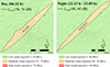 |
Figure 1. Sound exposure ranges for GVA2017: Day (06–22 h) – low (< 50 dBA), moderate (50–70 dBA), high (> 70 dBA); Night (22–23 h / 23–05 h) – low (< 40 dBA), moderate (40–60 dBA), high (> 60 dBA). |
-
Low sound exposure: Sound levels in this range are below 50 dBA, representing areas relatively far away from any air traffic routes. The limit of 50 dBA approximately corresponds to the recommendations by WHO for the Day-Evening-Night Level (Lden) of 45 dBA [2], given that Lden is some 2 dB larger than the corresponding Lday [30].
-
Moderate sound exposure: Sound levels in this range are between 50 and 70 dBA, representing areas in proximity to the airport and/or departure or approach flight corridors.
-
High sound exposure: Sound levels in this range are above 70 dBA, representing areas very close to the runway such as airport premises or nearby airport buildings.
To allow for reliable nighttime (22–23 h and 23–05 h) comparisons, the sound exposure ranges are reduced by 10 dB (see Fig. 1 right).
2.5. Annual aircraft noise exposure calculation with sonAIR: Workflow
This section outlines the five key steps (Sects. 2.5.1–2.5.5) for calculating annual aircraft noise exposure with sonAIR. For a detailed explanation of the calculation process, see [4]. While GVA Airport is used for demonstration, the workflow applies similarly to other airports.
2.5.1. Project setup and data import into the GIS environment
Initialized in the GIS environment with 25 m × 25 m digital terrain and ground cover data, the runway system is defined by endpoint coordinates and designators (e.g., here 04–22). To optimize calculations, the area is divided into 4 km × 4 km computation tiles for parallel processing, though tiles at the edges of the calculation area may have smaller dimensions. Receiver points are placed on a 150 m × 150 m grid, and flight trajectories are imported. Figure 2 (left) illustrates ground cover data and tiles after trajectory import.
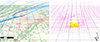 |
Figure 2. Ground cover data and computation tiles displayed after importing the flight trajectories (left). Receiver point of interest (red point) shown after the cell grid point generation (right). The cell grid points indicate virtual source positions. For each source-receiver combination a sound propagation calculation is performed and stored in a database. |
The airport data, including radar data and air traffic movement lists, is processed in two steps. First, movements are analyzed by tail number to generate statistics by aircraft type, route, and time period (06–22 h, 22–23 h, 23–05 h). Second, radar data is validated, smoothed, and extended to the runway. As sonAIR requires N1 as an input, this is derived from the processed trajectories using a method developed at the authors’ institution [13]. Table 3 provides input data and key calculation figures for GVA Airport for the year 2017.
Key figures of the setup of the sonAIR project for GVA2017 in the GIS environment.
For the current calculation, up to 200 flight trajectories per aircraft type, air route, and time period are selected through a randomized statistical selection (i.e., all flights if less than 200 flights took place), resulting in approximately 43 000 flight trajectories for GVA2017.
2.5.2. Cell grid generation and attenuation database precalculation
The airspace is divided into cells based on the imported flight trajectories, as aircraft generally follow consistent routes annually. To minimize repetitive calculations, sound attenuation is precalculated using sonX [14] at cell corners along these routes, where virtual source positions are placed for the sound propagation calculation. During single flight simulations (see Sect. 2.5.3), these precalculated values are used, weighted by the aircraft position within the cell. Cell sizes are dynamically adjusted based on altitude and horizontal distance to receivers [4]. Once the attenuation database is established, demanding a large initial effort, it can be reused for future calculations, and incrementally extended if necessary with new cell grid points based on additional flight routes and/or trajectories, significantly speeding up subsequent annual calculations. However, changes in input data, such as updated ground cover data, or calculation settings, require a complete recalculation. Figure 2 (right) shows the cell corner points for the single receiver setup in the yellow tile, with reduced grid points further away.
To manage the complexity of sound propagation calculations, sonX uses a hybrid modelling approach. Forhigh-altitude aircraft with direct and unshielded sound propagation paths, “on-the-fly” attenuation is calculated during simulations, without precalculating cell grid points. In complex propagation situations, attenuation values are precalculated. The simplified model applies when the aircraft angle exceeds 15° above the horizon. Figure 3 illustrates simple versus complex propagation, while Figure 2 (right) shows cell grid generation and precalculation below the 15° threshold.
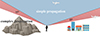 |
Figure 3. Hybrid modeling approach with line of sight above horizon (obstacles, i.e., terrain and/or buildings) including a 15° off-set as criterion to distinguish between simple and complex propagation situations. |
In this study, separate attenuation databases were computed for each version A–D, as shown in Table 2, with approximately 4 million cell grid points for GVA. The precalculation of attenuation for an airport the size of GVA requires approximately two weeks and was performed mainly on two systems: one with an Intel® Xeon® W-2155 CPU (3.30 GHz, 10 cores) and another with an Intel® Xeon® W-2275 CPU (3.30 GHz, 14 cores). Additional support, partly available due to being a shared resource, came from a machine with two Intel® Xeon® Gold 6248R CPUs (3.00 GHz, 24 cores each), ensuring efficient parallel processing. Incremental attenuation calculation, such as incorporating new flight routes or trajectories, take at most a few days, depending on the number of newly generated cell grid points. To handle this computational load efficiently, calculations are parallelized using the predefined computation tiles.
2.5.3. Single flight simulation
Once the attenuation database is precalculated, the so-called “noise footprints” are simulated. Footprints are receiver grids of the energetically averaged mean sound exposure level (LAE or LAS, max) for a representative number of flights of a specific aircraft/engine type on a certain air route during a given time period. The values are scaled to reflect one aircraft movement of a specific aircraft type along a specific air route (accounting for flight dispersion over a number of flights) during a specific time period and are referenced to 1 s (for L AE) (see, e.g. [31]).
To calculate these footprints, individual flight simulations are executed for all imported flight trajectories. These trajectories are categorized based on aircraft/engine type, air route, and time period, as previously defined. A time-step approach is employed, where the sound source model moves along the flight trajectory in discrete time intervals, usually of 1 s. Figure 4 shows cell grid points for a single flight path (left) and a noise footprint for a specific aircraft type and route over a defined period, with brightness indicating noise exposure levels (right).
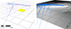 |
Figure 4. Precalculated cell grid points (attenuations) used for a single flight path (left) and resulting “noise footprint” for multiple flights of a specific aircraft/engine type on a given route during a specified time period (right). |
2.5.4. Substitution
For annual aircraft noise calculations, sonAIR requires emission models for all major aircraft types appearing in the list of movements. However, not all aircraft types have corresponding emission models. To address this issue, a substitution method is used, following the approach detailed in [32]. Using this approach, aircraft types without an emission model are matched with a proxy type, i.e., similar aircraft types for which emission models are available. Differences in noise emission between the missing and proxy types are corrected based on official certification levels in the following superposition (decibel adjustment). This method maintains the accuracy of noisecalculations despite the limited number of available emission models.
2.5.5. Superposition
In the final step, yearly noise exposures are calculated (L Aeq, L den). To that aim, the aircraft type, flight route, and time period specific footprints are weighted by the number of aircraft movements derived from the movement list (Sect. 2.5.1). The weighted footprints are then energetically summed and averaged over the duration of the time period of interest. This yields the total annual aircraft noise exposure, in our study represented as theA-weighted equivalent continuous sound pressure level L Aeq, for all operating times of interest.
2.6. Presentation of the aircraft noise scenario
As this study focuses on the aircraft noise scenario at GVA Airport for the year 2017, specifically during the daytime period (06–22 h), this section details the scenario specific to the airport.
The study area is located in southwestern Switzerland, with GVA Airport positioned north of Geneva, near the Swiss-French border. The airport features a single runway (04–22) oriented southwest to northeast, with Lake Geneva situated to the east. Figure 5 provides a cartographic representation of the area, including the total calculation area covering 54 km by 57 km (3078 km2) outlined as a red rectangle.
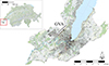 |
Figure 5. Top left: Overview map showing the location of GVA in Switzerland. Large map: Detailed cartographic overview of the study area. Basemap: Swiss Map Raster 10, Federal Office of Topography swisstopo. |
The year 2017 is selected to assess the sensitivity of calculation settings on sonAIR results and compare them with the best-practice model for a yearly noise exposure. This year, unaffected by COVID-19, provides a scenario without pandemic-related variations in traffic or operations. Calculations focus on large commercial aircraft, excluding general aviation (maximum take-off weight MTOW < 8618 kg), as its contribution to overall aircraft noise exposure is small.
The time periods are defined according to Swiss legislation [33]: daytime (06–22 h), first (22–23 h), second(23–24 h) and last (05–06 h) hour of the night (negligible air traffic, thus not further discussed). There is a flight ban from 23:30–05:00 h for Swiss airports. Table 4 displays the number of aircraft movements for GVA during the exposure year 2017 for the daytime period 06–22 h.
Annual number of movements of large aircraft in 2017 for GVA for the calculated time periods.
Details of aircraft movements for other time periods are provided in the Appendix . Calculations cover all specified time periods. Furthermore, air traffic scenarios for GVA (2019), ZRH (2017 and 2019), and SANC-TE are detailed in Appendices A and B. The primary focus of this paper, however, is on GVA for 2017 during the daytime period (06–22 h) for analysis and comparisons, specifically presenting the day’s equivalent continuous sound pressure level L Aeq.
3. Results
Section 3.1 evaluates the sonAIR versions B to D against the baseline version A (see Tab. 2), while Section 3.2 compares the sonAIR versions A to D against official calculations performed using the best-practice model FLULA2 (see Sect. 2.4). The results focus on GVA Airport for the year 2017 during daytime period 06–22 h, with geographical and statistical assessments of differences across the sound exposure ranges.
Comparisons for nighttime periods are included in the supplementary material (Sect. S1). Furthermore, comparisons for GVA Airport for the year 2019, ZRH Airport for the years 2017 and 2019, and SANC-TE airport can also be found in the supplementary material (Sects. S2–S3).
3.1. sonAIR versus sonAIR
Figure 6B shows the difference between sonAIR with grassland and the baseline with ground cover. Ground cover affects sound propagation, causing local variations from −3.5 dB to +9.3 dB. However, average deviations are small, mostly between 0 and +0.2 dB across the entire sound exposure range (Fig. 7), with slightly higher sound exposure levels overall when using grassland. Positive differences of the sound exposure levels are observed in forested areas, particularly north of the airport (Fig. 6A), where the assumption of purely grassland neglects the excess attenuation provided by trees. Over Lake Geneva, negative differences are found as the water body alters ground effect and leads to higher sound exposure level, when taken into account. Similar deviations are seen in urban areas with hard ground surfaces, though this is not a consistent pattern. Generally, as the phase-sensitive ground effect calculation produces a spectral interference pattern in dependence of geometry and ground properties, a change of ground properties can cause a level increase or decrease at a specific frequency and the effect on the A-weighted level can either be positive or negative. Exemplarily, this is shown in Figure C.1 in the appendix, where grassland produces a distinct dip at 160 Hz and an amplification at 400 Hz, whereas actual ground cover results in a smoother frequency spectrum. Given the dominant aircraft noise frequencies, this ground effect leads to higher noise exposure with grassland.
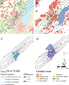 |
Figure 6. Individual sonAIR versions for GVA2017 during 06–22 h time period: (A) sonAIR contours with detailed ground cover, (B) sonAIR contours with grassland, (C) sonAIR contours with detailed ground cover and buildings, (D) sonAIR contours with detailed ground cover and METEO. For (B)–(D), grid differences (new version minus baseline version A) and resulting contours for each version are shown. |
 |
Figure 7. Statistical summary of differences for GVA2017 during 06–22 h time period, including mean and interpercentile range (IPR) – the range between the 2.5th and 97.5th percentiles, capturing 95% of the data –, as well as overall mean (μ), standard deviation (σ) and min/max values, across low, moderate, and high sound exposure levels. |
Figure 6C shows the difference between the sonAIR version including shielding by buildings within airport premises and the sonAIR baseline version without shielding. Buildings cause significant sound reductions, particularly within 2–3 km of the runway. This effect is strongest to the south of the runway, where larger buildings are located, and is most pronounced in the 50–70 dB range, with the largest reductions around 64 dB (Fig. 7). Outside this range, differences are minimal.
Figure 6D shows the difference between sonAIR METEO (accounting for acoustic shadow zones under unfavorable conditions) and the sonAIR baseline version without these effects. Meteorological effects are strongest within 2–4 km of the runway, where aircraft are on or near the ground. Reductions in sound levels due to meteorological conditions increase with noise levels above 50 dB. The mean reduction is −0.4 dB in the 50–70 dB range and −1.0 dB for levels above 70 dB (Fig. 7). Below 50 dB, meteorological effects are negligible as the aircraft determining the noise exposure are already high above ground and the sound incidence angles are steep.
3.2. sonAIR versus best-practice model FLULA2
Figure 8A compares sonAIR with ground cover with the official calculation using the current best-practice model FLULA2. The detailed calculation including ground cover in sonAIR results in considerable local spatial differences, ranging from −13.9 dB to +5.2 dB (see Fig. 9). In the 50–70 dB range, sonAIR yields slightly lower sound levels, with a mean difference of −0.4 dB, while for levels below 50 dB, the differences balance out (0.0 dB). Overall, sonAIR tends to yield lower sound levels than the best-practice model, especially for high noise exposures.
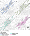 |
Figure 8. sonAIR versions for GVA2017 during 06–22 h time period: (A) sonAIR with detailed ground cover, (B) sonAIR with uniform grassland, (C) sonAIR with detailed ground cover and buildings, (D) sonAIR with detailed ground cover and METEO. The resulting noise contours are compared to the contours of the current best-practice model FLULA2. |
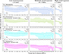 |
Figure 9. Statistical summary of differences for GVA2017 during 06–22 h time period, including mean and interpercentile range (IPR) – the range between the 2.5th and 97.5th percentiles, capturing 95% of the data –, as well as overall mean (μ), standard deviation (σ) and min/max values across low, moderate, and high sound exposure levels. |
Figure 8B compares sonAIR with uniform grassland with those yielded by FLULA2. The results are more similar than when using detailed ground cover, as both models assume uniform grassland. This is particularly evident in the low and moderate sound exposure ranges, where the mean difference is predominantly close to 0.0 dB, with smaller standard deviations of the differences compared to using detailed ground cover (Fig. 9).
Figure 8C compares the sonAIR version accounting for shielding by buildings and the best-practice model FLULA2, which does not account for any shielding effects. Similar to the previous comparison as shown in Figure 6, major shielding effects and thus differences are observed in areas directly adjacent to the runway, with average differences of −1.0 dB or more in the 60–70 dB range and local reductions of up to −21.3 dB. Outside this range, shielding has only a minor effect, and differences between the models are similar to other sonAIR versions. Note that also positive differences between sonAIR and FLULA2 locally occur, which, however, are due to other differences in the calculations of sonAIR and FLULA2 (see Tab. 1) and not related to the shielding by buildings.
Figure 8D compares sonAIR METEO, which accounts for acoustic shadow zones, with the best-practice model FLULA2, which accounts for these effects in simplified manner using the empirical lateral attenuation correction. The impact of meteorological conditions is especially visible in areas close to the airport, i.e., 2–4 km laterally from the airport and in the moderate to high sound exposure ranges, with a mean reduction of −0.8 dB and −1.7 dB, respectively (Fig. 9). In the low exposure range, these effects are negligible, with differences similar to those of sonAIR version withoutMETEO.
Table 5 compares the results of the four sonAIR versions (ground cover, grassland, buildings, METEO) with those of the best-practice model FLULA2 for the sound exposure ranges low, moderate, high and the time periods (06–22 h, 22–23 h, 23–05 h). The metrics include mean difference (μ), standard deviation (σ), minimum, and maximum differences.
Statistical summary comparing the calculated sonAIR versions for GVA2017 and the best-practice model across all sound exposure levels (low, moderate, high) and time periods (06–22 h, 22–23 h, 23–05 h). Mean (μ), standard deviation (σ), minimum (min), and maximum (max) differences are presented.
Mean differences are generally small for the daytime period 06–22 h, ranging from 0.0 to −1.7, with the METEO version showing the largest difference for high exposure. Standard deviations vary moderately, peaking at 1.9 dB in the sonAIR version accounting for shielding for moderate sound exposure. Minimum values show extreme negative differences, particularly when accounting for shielding (−21.3 dB), while maximum values are similar for all versions per exposure range and take values between 0.2 and 5.2. In summary, the results show that, although deviations exist between the sonAIR versions and the best-practice model, the overall differences are moderate, with the sonAIR versions METEO and with buildings showing the largest differences to FLULA2 in noise exposure modeling.
Table 6 compares noise contour areas of the calculated sonAIR versions with the best-practice model FLULA2. For a structured evaluation, the focus is on 60, 65, and 70 dB noise contours for the daytime period and 50, 55, and 60 dB noise contours for the nighttime periods. The results show that the calculations of sonAIR producesimilar, but slightly differing noise extents. The largest deviations to FLULA2 are observed when accounting for buildings and meteorological conditions, as well as at lower sound levels during nighttime periods.
Appendix A and the supplementary material (Sects. S1–S3) provide comparisons of additional calculations performed with the BASIC module for GVA Airport (2019), ZRH Airport (2017 and 2019) and in both BASIC and METEO module for SANC-TE. The main findings from these comparisons are consistent with the results presented here, reinforcing the generalizability of the study’s conclusions.
Total areas of the resulting noise contours for the calculated sonAIR versions and the best-practice model (in km2) at considered sound exposure levels (Daytime period: 60–70 dBA, Nighttime periods: 50–60 dBA).
4. Discussion
In this study, we compare different sonAIR versions, each utilizing distinct input data and settings, both against each other and against the best-practice model FLULA2. The comparison focuses on annual aircraft noise scenarios at GVA Airport for the year 2017. The study is conducted to replace FLULA2 with sonAIR for the calculation of annual noise maps for Swiss airports and to decide on the appropriate settings in sonAIR. As FLULA2 and sonAIR represent two different generations of aircraft noise models, the discussion, which source and propagation effects should be taken into account in future aircraft noise models, is of broader interest.
The physics-based ground effect model of sonAIR introduces more local variability and thus less smoother noise contours, compared to FLULA2. This might be seen as a disadvantage from a practical point of view. However, the resulting gain in accuracy and the fact that local conditions are taken into account, increases credibility and acceptance of the results by the population. The full potential of a sophisticated sound propagation calculation can only be exploited, when combining it with detailed input data. Using detailed ground properties instead of assuming purely grassland results in systematic local changes in sound exposure, most prominently visible around GVA Airport for forested areas and water bodies. Even though the differences might be small on average, they can be very substantial locally. Consequently, it is recommended to use sonAIR with detailed ground properties.
In contrast to best-practice models, sonAIR offers the possibility to consider the effect of buildings. When incorporating shielding effects from buildings, the differences behind the buildings were considerable, but locally very limited and aligned with ground-level sources. Further, it is important to also account for reflections. While previous studies [23, 24] have shown that reflections have a smaller impact compared to shielding, they still contribute to overall noise levels. Accounting for buildings when calculating noise contours, creates irregular “noise islands” around buildings (Fig. C.2 in appendix). The coarse receiver grid (150 m × 150 m), similar in size to buildings, contributes to this irregularity. A finer grid improves accuracy, but this would increase the computational effort and be impractical for large-scale annual aircraft noise assessments. This suggests that, similar to the conclusions by Ramseier et al. [24], buildings may be of interest for special investigations, when receiver points on facades are calculated, while they are not to be recommended for large-scale noise mapping (e.g., annual aircraft noise scenarios).
Meteorological effects are most prominent close to the airport, where aircraft are either on the ground or at low altitudes, leading to small source-receiver angles. These conditions, known as grazing sound incidence [28], promote the formation of acoustic shadow zones and barrier effects. Results for GVA17 align with those obtained for an idealized airport, the standardized test environment SANC-TE, as detailed in Appendix B.
The meteorological effects revealed within this study are relatively large and may be less pronounced in other scenarios due to several factors. First, the single-runway configuration of GVA Airport allows for shadow zones adjacent to the runway, whereas at more complex airports with multiple intersecting runways, such as Zurich Airport (ZRH), these effects would be less significant. Second, the meteorological effects were quantified for daytime conditions. During the night, as discussed in Section 2.3, unfavorable meteorological conditions, and thus acoustic shadow zones, are less frequent, leading to smaller effects. Table 5 shows the impact of the Meteo version, including nighttime periods. During the day in the moderate sound exposure range, the Meteo version reduces average sound exposure by −0.8 dB compared to the best-practice model, while at night the reduction is smaller, at −0.1 dB. Notably, the lateral attenuation in the best-practice programs does not sufficiently account for this effect.
Incorporating meteorological effects requires the addition of an attenuation database, which approximately doubles the computational time. In the example of GVA17, the calculation time increases from 2 weeks (using only the BASIC module) to 4 weeks when both BASIC and METEO modules are included. The extra effort does not seem justified in comparison to the importance of the effect. Therefore, including meteorology for large-scale noise mapping is not recommended.
5. Conclusion
In this study, a series of calculations were performed using sonAIR for Geneva and Zurich Airports for the years 2017 and 2019 and for a hypothetical, idealized airport. The study reveals that there are mostly minor differences over a wide exposure range between sonAIR as a next-generation model and FLULA2 as a typical representative best-practice model, given that effects not accounted for by FLULA2 (METEO, shielding by buildings) also remain unaccounted for by sonAIR. However, locally there can be large differences which can be attributed to the more physics-based model of sonAIR. sonAIR offers a more accurate representation of real-world conditions, which results in less smooth noise contours than with best practice models.
For large-scale noise mapping, effects which sonAIR can account for, namely, meteorological conditions and shielding by buildings, may not be relevant or even not purposeful for noise mapping. Therefore, we recommend the following input data and parameter settings for large-scale noise assessments such as annual aircraft noise calculations with sonAIR: sound propagation calculations assuming a homogeneous atmosphere with detailed ground cover properties, without buildings (i.e., BASIC module only). The modular design of sonAIR, however, enables control over the level of detail based on computational demands, allowing for more precise calculations and the inclusion of additional effects for more detailed analyses.
GVA: Empa report 5214.018331, ZRH: Empa report 5214.018332
Acknowledgments
This work was funded by the Swiss Federal Office of the Environment FOEN (Assignment No. 5214028869), Zurich Airport and The Office of Mobility and Transport of Zurich (Assignment No. 5214025794), and Geneva Airport (Assignment No. 5214020920). Portions of this work have been previously published as a conference paper [10]. The authors would like to thank Geneva and Zurich Airports for permission to use and present the data for this study.
Data availability statement
The data are available from the corresponding author on request.
Supplementary material
Supplementary file provided by the authors. Access Supplementary Material
References
- L. Jarup, W. Babisch, D. Houthuijs, G. Pershagen, K. Katsouyanni, E. Cadum, M.-L. Dudley, P. Savigny, I. Seiffert, W. Swart, O. Breugelmans, G. Bluhm, J. Selander, A. Haralabidis, K. Dimakopoulou, P. Sourtzi, M. Velonakis, F. Vigna-Taglianti: Hypertension and exposure to noise near airports: the HYENA study. Environmental Health Perspectives 116, 3 (2007) 329–333. [Google Scholar]
- WHO: Environmental noise guidelines for the European region. [Online]. Available: https://www.who.int/europe/publications/i/item/9789289053563. [Google Scholar]
- C. Zellmann, B. Schäffer, J.M. Wunderli, U. Isermann, C. Paschereit: Aircraft noise emission model accounting for aircraft flight parameters. Journal of Aircraft 55, 2 (2018) 682–695. [CrossRef] [Google Scholar]
- J.M. Wunderli, C. Zellmann, M. Köpfli, M. Habermacher: sonAIR – a GIS-integrated spectral aircraft noise simulation tool for single flight prediction and noise mapping. Acta Acustica United with Acustica 104, 3 (2018) 440–451. [Google Scholar]
- D. Jäger, C. Zellmann, F. Schlatter, J.M. Wunderli: Validation of the sonAIR aircraft noise simulation model. Noise Mapping 8, 1 (2021) 95–107. [Google Scholar]
- J. Meister, S. Schalcher, J. M. Wunderli, D. Jäger, C. Zellmann, B. Schäffer: Comparison of the aircraft noise calculation programs sonAIR, FLULA2 and AEDT with noise measurements of single flights. Aerospace 8, 12 (2021) 388. [Google Scholar]
- W. Krebs, R. Bütikofer, S. Plüss, G. Thomann: Sound source data for aircraft noise simulation. Acta Acustica United with Acustica 90, 1 (2004) 91–100. [Google Scholar]
- W. Krebs, R. Büttikofer, G. Thomann: FLULA2, ein verfahren zur berechnung und darstellung der fluglärmbelastung. technische programm-dokumentation. Version 4. [Google Scholar]
- U. Department of Transportation: Washington, DC. Aviation environmental design tool (AEDT) version 3c. Technical manual. [Google Scholar]
- S. Schalcher, C. Zellmann, J. Meister, J.M. Wunderli, B. Schäffer: Calculation of annual aircraft noise exposure for geneva and zurich airports with the next-generation program sonAIR – first results, in: INTER-NOISE and NOISE-CON Congress and Conference Proceedings. Vol. 265, 2023, pp. 1124–1132. [Google Scholar]
- B. für Umwelt (BAFU), B. für Zivilluftfahrt(BAZL), B.U.S.V.G.V. Generalsekretariat des Eidg: Departementes für Verteidigung. Leitfaden fluglärm. [Online]. Available: https://www.bafu.admin.ch/bafu/de/home/themen/thema-laerm/laerm--publikationen/publikationen-laerm/leitfaden-fluglaerm.html. [Google Scholar]
- W. Krebs, M. Balmer, E. Lobsiger: A standardised test environment to compare aircraft noise calculation programs. Applied Acoustics 69, 11 (2008) 1096–1100. [Google Scholar]
- O. Schwab, C. Zellmann: Estimation of flight-phase-specific jet aircraft parameters for noise simulations. Journal of Aircraft 57, 6 (2020) 1111–1120. [Google Scholar]
- J.M. Wunderli, B. Schäffer: Dokumentation des sonX ausbreitungsmodells. programmversion: sonRAIL v6.0.0 bzw. sonARMS v5.0.0 bzw. sonAIR v3.0.0. [Online]. Available: https://www.empa.ch/de/web/s509/sonx. [Google Scholar]
- International Organisation for Standardization (ISO): ISO 9613-2. [Online]. Available: https://www.iso.org/standard/20649.html. [Google Scholar]
- J. Defrance, E. Salomons, I. Stuijt, D. Heimann, B. Plovsing, G. Watts, H. Jonasson, X. Zhang, E. Premat, I. Schmich-Yamane, F.-E. Aballéa, M. Baulac, F. Roo: Outdoor sound propagation reference model developed in the european harmonoise project. Acta Acustica United with Acustica 93, 2 (2007) 213–227. [Google Scholar]
- Z. Maekawa: Noise reduction by screens. Applied Acoustics 1, 3 (1968) 157–173. [Google Scholar]
- A.D. Pierce, P.W. Smith: Acoustics: an introduction to its physical principles and applications. Physics Today 34, 12 (1981) 56–57. [Google Scholar]
- K. Heutschi: Calculation of reflections in an urban environment. Acta Acustica United with Acustica 95, 4 (2009) 644–652. [Google Scholar]
- J.M. Wunderli: An extended model to predict reflections from forests. Acta Acustica United with Acustica 98, 2 (2012) 263–278. [Google Scholar]
- J.-M. Wunderli: Modelling reflections from single trees and entire forests, in: Integrating 4th EAA Euroregio 2019, 9–13 September 2019. RWTH Aachen University, 2019, p. 9. [Online]. Available: http://publications.rwth-aachen.de/record/769227. [Google Scholar]
- R. Pieren, J.M. Wunderli: A model to predict sound reflections from cliffs. Acta Acustica United with Acustica 97, 2 (2011) 243–253. [Google Scholar]
- F. Schlatter, M. Köpfli, J.M. Wunderli: Relevance of buildings in aircraft noise predictions, in: INTER-NOISE and NOISE-CON Congress and Conference Proceedings. Vol. 258, 2018, pp. 3042–3051. [Google Scholar]
- T. Ramseier, S. Schalcher, J.M. Wunderli, B. Schäffer: Impact of buildings, forests and cliffs on aircraft noise mapping: case study. Transportation Research Part D: Transport and Environment 133 (2024) 104279. [Google Scholar]
- C. Wu, S. Redonnet: Aircraft noise impact prediction with incorporation of meteorological effects. Transportation Research Part D: Transport and Environment 125 (2023) 103945. [CrossRef] [Google Scholar]
- C. Zellmann, J.M. Wunderli: Influence of the atmospheric stratification on the sound propagation of single flights, in: INTER-NOISE and NOISE-CON Congress and Conference Proceedings, Vol. 249, 2014, pp. 3770–3779. [Google Scholar]
- SAE: AIR5662: method for predicting lateral attenuation of airplane noise – SAE international. [Online]. Available: https://www.sae.org/standards/content/air5662/. [Google Scholar]
- J.M. Wunderli, J. Meister, D. Jäger, S. Schalcher, C. Zellmann, B. Schäffer: Aircraft noise in situations with grazing sound incidence – comparing different modeling approaches. The Journal of the Acoustical Society of America 151, 5 (2022) 3140–3151. [Google Scholar]
- H. Feng, Y. Zhou, W. Zeng, C. Ding: Review on metrics and prediction methods of civil aviation noise. International Journal of Aeronautical and Space Sciences 24, 5 (2023) 1199–1213. [Google Scholar]
- M. Brink, B. Schäffer, R. Pieren, J.M. Wunderli: Conversion between noise exposure indicators Leq24h, LDay, LEvening, LNight, Ldn and Lden: principles and practical guidance. International Journal of Hygiene and Environmental Health 221, 1 (2018)54–63. [Google Scholar]
- B. Schäffer, R. Bütikofer, S. Plüss, G. Thomann: Aircraft noise: accounting for changes in air traffic with time of day. The Journal of the Acoustical Society of America 129, 1 (2011) 185–199. [Google Scholar]
- European Civil Aviation Conference (ECAC): ECAC.CEAC doc 29: report on standard method of computing noise contours around civil airports. Applications guide, 4th edn. Vol. 1, 2016. [Online]. Available: https://www.ecac-ceac.org/documents/ecac-documentsand-international-agreements. [Google Scholar]
- Noise abatement ordinance (NAO) from 15 December 1986 (status as of 1 November 2024). [Online]. Available: http://www.admin.ch/ch/d/sr/8/814.41.de.pdf. [Google Scholar]
Appendix A
GVA2017, GVA2019, ZRH2017 and ZRH2019
Tables A.1 and A.2 show key figures of the sonAIR projects for GVA2017, GVA2019, ZRH2017 and ZRH2019 and statistical summary of their comparisons with the best-practice model.
Key figures of the setup of the sonAIR projects for GVA2017, GVA2019, ZRH2017 and ZRH2019.
Statistical summary comparing sonAIR BASIC mode for GVA (2019) and ZRH (2017, 2019) with the best-practice model across all sound exposure levels (low, moderate, high) and time periods (06–22 h, 22–23 h, 23–05 h). Mean (μ), standard deviation (σ), minimum (min), and maximum (max) differences are shown.
Appendix B
Swiss Aircraft Noise Test Environment (SANC-TE)
The Swiss Aircraft Noise Test Environment (SANC-TE) consists of a virtual airport centered within the calculation area, featuring a single runway. A sinusoidal terrain ridge runs parallel to the runway in the northern region, while a rotationally symmetric hill is present in the southwestern area. These terrain features allow for the assessment of terrain-induced shielding and ground effects. The entire area is modeled as grassland. Flight trajectories account for lateral track dispersion, with a total of 175 187 aircraft movements considered. For further details, see [12]. Tabs. B.1 and B.2 show key figures of the sonAIR project for SANC-TE and statistical summary of the comparison with the best-practice model.
Key figures of the setup of the sonAIR project for SANC-TE.
Statistical summary comparing sonAIR versions BASIC and METEO with the best-practice model for SANC-TE airport across sound exposure levels (low, moderate, high) and for 06–22 h time period. Mean (μ), standard deviation (σ), minimum (min), and maximum (max) differences are shown.
Appendix C
Additional plots
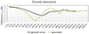 |
Figure C.1. Ground attenuation for grassland and actual ground cover for an exemplary receiver point at GVA. Positive values indicate attenuation, while negative values indicate amplification of the sound exposure. |
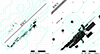 |
Figure C.2. Situation of GVA with the buildings close to the runway, with the red points indicating the receiver grid and the line the resulting contours. Left: Overview, Right: Enlarged view of the same situation. The irregular patterns in the noise contours are due to some receiver points being completely shielded from the runway, while others are not shielded at all. |
Cite this article as: Schalcher S. Zellmann C. Wunderli J.-M. & Schäffer B. 2025. Assessing the influence of ground cover, buildings and meteorological conditions on annual aircraft noise exposure: sensitivity study with the simulation tool sonAIR. Acta Acustica, 9, 54. https://doi.org/10.1051/aacus/2025035.
All Tables
Key figures of the setup of the sonAIR project for GVA2017 in the GIS environment.
Annual number of movements of large aircraft in 2017 for GVA for the calculated time periods.
Statistical summary comparing the calculated sonAIR versions for GVA2017 and the best-practice model across all sound exposure levels (low, moderate, high) and time periods (06–22 h, 22–23 h, 23–05 h). Mean (μ), standard deviation (σ), minimum (min), and maximum (max) differences are presented.
Total areas of the resulting noise contours for the calculated sonAIR versions and the best-practice model (in km2) at considered sound exposure levels (Daytime period: 60–70 dBA, Nighttime periods: 50–60 dBA).
Key figures of the setup of the sonAIR projects for GVA2017, GVA2019, ZRH2017 and ZRH2019.
Statistical summary comparing sonAIR BASIC mode for GVA (2019) and ZRH (2017, 2019) with the best-practice model across all sound exposure levels (low, moderate, high) and time periods (06–22 h, 22–23 h, 23–05 h). Mean (μ), standard deviation (σ), minimum (min), and maximum (max) differences are shown.
Statistical summary comparing sonAIR versions BASIC and METEO with the best-practice model for SANC-TE airport across sound exposure levels (low, moderate, high) and for 06–22 h time period. Mean (μ), standard deviation (σ), minimum (min), and maximum (max) differences are shown.
All Figures
|
Figure 1. Sound exposure ranges for GVA2017: Day (06–22 h) – low (< 50 dBA), moderate (50–70 dBA), high (> 70 dBA); Night (22–23 h / 23–05 h) – low (< 40 dBA), moderate (40–60 dBA), high (> 60 dBA). |
| In the text | |
|
Figure 2. Ground cover data and computation tiles displayed after importing the flight trajectories (left). Receiver point of interest (red point) shown after the cell grid point generation (right). The cell grid points indicate virtual source positions. For each source-receiver combination a sound propagation calculation is performed and stored in a database. |
| In the text | |
|
Figure 3. Hybrid modeling approach with line of sight above horizon (obstacles, i.e., terrain and/or buildings) including a 15° off-set as criterion to distinguish between simple and complex propagation situations. |
| In the text | |
|
Figure 4. Precalculated cell grid points (attenuations) used for a single flight path (left) and resulting “noise footprint” for multiple flights of a specific aircraft/engine type on a given route during a specified time period (right). |
| In the text | |
|
Figure 5. Top left: Overview map showing the location of GVA in Switzerland. Large map: Detailed cartographic overview of the study area. Basemap: Swiss Map Raster 10, Federal Office of Topography swisstopo. |
| In the text | |
|
Figure 6. Individual sonAIR versions for GVA2017 during 06–22 h time period: (A) sonAIR contours with detailed ground cover, (B) sonAIR contours with grassland, (C) sonAIR contours with detailed ground cover and buildings, (D) sonAIR contours with detailed ground cover and METEO. For (B)–(D), grid differences (new version minus baseline version A) and resulting contours for each version are shown. |
| In the text | |
|
Figure 7. Statistical summary of differences for GVA2017 during 06–22 h time period, including mean and interpercentile range (IPR) – the range between the 2.5th and 97.5th percentiles, capturing 95% of the data –, as well as overall mean (μ), standard deviation (σ) and min/max values, across low, moderate, and high sound exposure levels. |
| In the text | |
|
Figure 8. sonAIR versions for GVA2017 during 06–22 h time period: (A) sonAIR with detailed ground cover, (B) sonAIR with uniform grassland, (C) sonAIR with detailed ground cover and buildings, (D) sonAIR with detailed ground cover and METEO. The resulting noise contours are compared to the contours of the current best-practice model FLULA2. |
| In the text | |
|
Figure 9. Statistical summary of differences for GVA2017 during 06–22 h time period, including mean and interpercentile range (IPR) – the range between the 2.5th and 97.5th percentiles, capturing 95% of the data –, as well as overall mean (μ), standard deviation (σ) and min/max values across low, moderate, and high sound exposure levels. |
| In the text | |
|
Figure C.1. Ground attenuation for grassland and actual ground cover for an exemplary receiver point at GVA. Positive values indicate attenuation, while negative values indicate amplification of the sound exposure. |
| In the text | |
|
Figure C.2. Situation of GVA with the buildings close to the runway, with the red points indicating the receiver grid and the line the resulting contours. Left: Overview, Right: Enlarged view of the same situation. The irregular patterns in the noise contours are due to some receiver points being completely shielded from the runway, while others are not shielded at all. |
| In the text | |
Current usage metrics show cumulative count of Article Views (full-text article views including HTML views, PDF and ePub downloads, according to the available data) and Abstracts Views on Vision4Press platform.
Data correspond to usage on the plateform after 2015. The current usage metrics is available 48-96 hours after online publication and is updated daily on week days.
Initial download of the metrics may take a while.