| Issue |
Acta Acust.
Volume 9, 2025
|
|
|---|---|---|
| Article Number | 66 | |
| Number of page(s) | 12 | |
| Section | Environmental Noise | |
| DOI | https://doi.org/10.1051/aacus/2025051 | |
| Published online | 21 October 2025 | |
Scientific Article
Advancing the characterization of urban acoustic environments through multimetric analysis
1
Department of Engineering Acoustics, Technische Universität Berlin, Einsteinufer 25, 10587 Berlin, Germany
2
Institute for Urban Public Health, University Medicine Essen, University Duisburg-Essen, Hufelandstr. 55, 45147 Essen, Germany
3
Research Group Landscape Ecology and Landscape Planning, Faculty of Spatial Planning, TU Dortmund University, August Schmidt Str. 10, 44227 Dortmund, Germany
* Corresponding author: This email address is being protected from spambots. You need JavaScript enabled to view it.
Received:
11
April
2025
Accepted:
10
September
2025
Abstract
Urbanization has intensified the complexity of acoustic environments, necessitating a more comprehensive understanding to support urban acoustic planning for healthier living spaces. Traditional noise monitoring, primarily based on sound pressure level indices, is insufficient for capturing the full scope of these environments. This study investigates whether a diverse set of acoustic metrics can improve the characterization of acoustic environments and examines their stability across different land use types. We analyzed 1 year of time-series data from acoustic monitoring stations in Bochum, Germany, calculating psychoacoustic, ecoacoustic, and complex network indices. Our goals were to: (1) identify interdependencies among selected metrics, (2) uncover temporal patterns in acoustic measurements, and (3) relate them to their respective locations. Methods included correlation analysis, DBSCAN (Density-Based Spatial Clustering of Applications with Noise) clustering, principal component analysis, and descriptive statistics with diurnal aggregation. The findings demonstrate that acoustic indices of eight distinct dimensions, along with eight individual metrics, reveal crucial temporal, spatial variations of the acoustic environment and the interplay of individual sound sources overlooked by conventional sound pressure level (SPL) metrics. In particular, the study identifies the maximum Sharpness (Aures method), Link Density, the Bioacoustic Index, and the Amplitude Index as the most effective predictors of land use types, achieving the highest Adjusted Rand Index values (0.25, 0.17, 0.13, 0.13). Incorporating such indices into acoustic monitoring practices offers a refined, site-sensitive framework to identify more nuanced qualities of the acoustic environment, therefore, potentially laying the groundwork for targeted urban interventions that could promote health.
Key words: Acoustic indices / Temporal patterns / Acoustic monitoring / Urban acoustic environments / Environmental acoustics
© The Author(s), Published by EDP Sciences, 2025
 This is an Open Access article distributed under the terms of the Creative Commons Attribution License (https://creativecommons.org/licenses/by/4.0), which permits unrestricted use, distribution, and reproduction in any medium, provided the original work is properly cited.
1 Introduction
The fast spread of urban areas is a continuous process that leads to greater environmental impacts [1]. Noise pollution, for example, affects over 95 million EU citizens who are exposed to levels considered harmful [2]. Addressing the challenge of creating healthier and more livable cities requires a strong focus on understanding the acoustic environment (AE). This is essential not only because noise pollution poses a significant health risk but also because the AE offers valuable information on various urban subsystems, such as biodiversity, traffic, and the built environment [3–5]. A deeper understanding of these dynamics can inform targeted interventions that not only mitigate the negative effects of sound but also foster the creation of spaces with restorative qualities, ultimately contributing to positive healthoutcomes [1].
While traditional noise abatement measures have focused mainly on reducing sound pressure levels (SPL) to improve AE, they often fail to account for the diverse events where specific sound sources that follow specific frequency patterns stand out and shape the real-life auditory experience of residents and its effects [6, 7]. The European noise directive (2002/49/EC) emphasizes noise mapping to guide urban development by displaying noise hotspots, for example, but these maps often fall short in reflecting the diversity of urban AE since they focus only on the main noise sources (road traffic, train, aircraft and industry) [6].
The acoustic environment (AE), as experienced by humans, is multifaceted: while certain AEs can be detrimental to health, others can promote psychological restoration. This duality makes acoustic design a powerful tool for enhancing urban well-being by minimizing harmful noise and amplifying beneficial sounds [8]. Understanding how these qualities manifest in real-life settings is critical for urban planners. Various tools for assessing perceived acoustic qualities exist and have been standardized, involving residents directly, as “local experts" through both surveys and observations and providing deeper insights into their individual experiences. However, such participatory methods can be financially expensive, time-consuming, are limited to small areas and susceptible to biases [9].
To capture the complexity of the urban acoustic environment, monitoring systems play a crucial role. This is not only common in urban contexts but also in ecoacoustics [10], where passive acoustic monitoring (PAM) has proven effective in ecosystem assessment [11]. Recent advancements include noise monitoring techniques for predicting acoustic comfort through sound event detection [12] and citizen science approaches to noise monitoring, which combine mixed-model predictive modeling with public participation [6, 13]. Such methods have also been applied in large-scale data collection efforts, like those tracking temporal sound patterns at fixed monitoring points in cities [14].
Psychoacoustics plays a central role in bridging the gap between cost-intensive processes and sound quality prediction by linking specific acoustic properties to human auditory perception [15]. Psychoacoustic parameters are modeled on the basis of empirical evidence to offer a more nuanced understanding of how sound is experienced beyond simple loudness levels [16, 17]. For instance, these parameters can help identify time-variant patterns and qualities correlated with the perceived timbre of the acoustic environment, which might correlate with natural sound sources [18]. Fostering the presence of this type of sound can be beneficial for general well-being in contrast to technologically produced sounds that are often perceived as moreannoying [19].
Driven by the fact that the combination of the mentioned indices scarcely has been used for a long-term analysis of acoustic data, this study seeks to apply and interpret a set of acoustic indices within a longitudinal noise monitoring project denominated SALVE (Acoustic Quality and Health in Urban Environments) in which PAM procedures where used in the urban realm. By integrating a large number of acoustic indices into time-series analyses, we aim to explore how they perform relative to traditional SPL indices and examine how a selected array of key representative metrics varies across different locations and environmental conditions, particularly looking at diurnal patterns, as seen in similar studies like [14] and [20]. A clustering analysis is used to better understand how these indices correlate with non-acoustic criteria, such as land use categories, thereby offering insights into the diversity and complexity of the acoustic environment.
The core objectives of this paper are articulated through the following research questions:
-
Do acoustic indices capture additional information about the acoustic environment beyond noise measures?
-
Which acoustic indices capture similar information about the acoustic environment?
By addressing these questions, this study aims to contribute to a more comprehensive understanding of urban acoustic environments and the potential of specific acoustic indices to improve acoustic monitoring and analysis. To this end, we applied a series of statistical procedures, including correlation clustering to uncover similarities among commonly used acoustic indices, dimensionality reduction to streamline a structured analysis of the data, and cluster validation to confirm the practical relevance and performance of the selected indices (overview on Fig. 1).
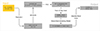 |
Figure 1 Methods used and outcome produced to address the research questions, the numbers in the brackets indicate the dimensions of the data structure, the first two steps we took in order to understand numerical overlap of the predefined set of indices, later we used PCA to select non-arbitrary indices as cluster representatives. This set of uncorrelated indices was then checked regarding sensitivity and response to the land use type where the device was positioned through a statistical procedure that included common clustering methods and the calculation of a validation metric. |
2 Material and methods
2.1 Acoustic monitoring framework and audio data
To address the research questions, data from the SALVE study is further analyzed [21]. Since this dataset covers a wide range of urban residential areas and a few large forested and designed green spaces, it is well-suited to our research aims. It contains data that was collected using 23 PAM-devices that created 3-minute recordings every 26 min, resulting in 50 recordings per day per device. Our selected data subset was collected from May 2019 to the end of May 2020 – a time span of more than a year (see Fig. 2). Each file was logged by a Wildlife Acoustic SM4 recorder with a SMMA2 microphone with a sampling frequency of 44.1 kHz and a 16-bit depth. The data has undergone several plausibility checks and has already been used in a number of publications [20, 22]. We used the existing features calculations, in particular the feature collection of ecoacoustic indices [23] and the Frequency-Correlation-Matrix (FCM)-based feature Link Density [24] and complemented this by adding differently weighted sound pressure levels and psychoacoustic parameters that were calculated for each audio file using the HEAD acoustics ArtemiS SUITE version 15.1. The data set finally amounted to 416,095 observation points of 98 calculated indices.
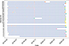 |
Figure 2 Overview of daily count of recordings for each device. The breaks between the dots represent a period of missing data, non-blue dots represent days with a total count of recordings < 50. |
2.2 Indices
Psychoacoustic metrics are used to quantify the human perception of sound. At the heart of psychoacoustic modeling is loudness, which takes into account physiological ear mechanisms, such as frequency-dependent hearing and masking processes [15]. Based on the loudness model, additional indices such as Sharpness, Roughness, Fluctuation Strength, and Tonality were derived and made accessible to the public in a standardized form (e.g., ISO 532-1, ECMA 418-2, DIN 45692).
We selected these psychoacoustic parameters to align closely with those used in established studies and standards in the field. For the sharpness parameter, we included two different versions: the standard metric defined in DIN 45692, and a loudness-weighted version proposed by Aures [25]. The latter is based on the idea that a higher overall loudness increases the perceived sharpness of a sound.
To face the variant character of sonic events, percentile values such as the 5th, 50th, and 95th percentiles are used. They provide insight into the distribution of these frame-based calculated psychoacoustic metrics over time. For example, the 95th percentile of Sharpness or Loudness captures the values above which only 5% of the observations occur, thereby, representing the louder, more prominent sound events within a measurement period [26, 27].
Furthermore, we decided to integrate the mean based on the root mean square of the signal samples since higher values are weighted using this procedure, the outcome is presumably closer to time-variant loudness-perception [28].
Our dataset also includes the Psychoacoustic Annoyance (PA) metric which combines multiple psychoacoustic parameters (Loudness N51, Sharpness, Roughness, and Fluctuation Strength) into a single measure, reflecting the general (psychoacoustic-) annoyance potential of a sound environment [15]. By weighting each parameter according to its contribution to perceived annoyance, the PA index is supposed to provide a comprehensive annoyance score, which could be more reflective of human perception than any single metric alone.
We incorporated well-established indices from the field of soundscape ecology all calculated using the R package “soundecology" [23], including the Acoustic Diversity Index (ADI) and the Acoustic Richness Index (AR), which are designed to quantify the diversity and intensity of acoustic signals within specific AE. Additionally, indices such as the Normalized Difference Soundscape Index (NDSI) and the Biocacoustic index (BIO) were employed to analyze intricate AEs, that are supposed to provide information about the composition of biophonic (natural) and anthrophonic (human-made) sound sources. To complete the set of ecoacoustic indices the Acoustic Complexity Index (ACI) was integrated which represents the mean band-variability of an acoustic signal.
From the ecoacoustic category we also utilized the Amplitude Index (M), a relative metric that captures the average dynamics of sound volume. This index is calculated as the ratio between the temporally weighted sound pressure level and its maximum values, providing information on the temporal variability and dynamic range of the AE.
To further enhance the quantification of spectral dominance, we integrated FCM-based indices. Among these, we used Link Density (LD) as a measure derived from the complex network of the FCMs. Higher values of LD indicate that an acoustic environment is more acoustically saturated resulting in a less diverse tempo-spectral outcome. This metric was also incorporated into our study to assure and discuss compatibility with a previous study [29].
Finally, we integrated widely used SPL indices. They were adjusted according to the internationally standardized A- and C-weighting curves (ISO 389-7:2019), which are inversions of equal loudness contours, established to reflect the non-linear sensitivity of humanhearing. This inclusion also ensures consistency with established methodologies and allows for comparisons between studies.
Another quantity of or dataset is kurtosis which is calculated as the 4th statistical moment of the amplitude of an audio signal. This dimensionless quantity describes the impulsiveness of a distribution relative to a normal distribution. The greater the amount of kurtosis, the more prominent impulse-like peaks are present in the signal [30].
A description of each indicator can be found in the supplementary material of [29] and [20].
2.3 Land use types
In order to carry out a location-based comparison of the measurements, calculation and validation of the clustering, we used land use types of the areas where the selected devices were positioned. We took over the land use definitions that where the result of a simple review process where several people examined 360° photos of the device locations separately. This approach was carried out due to a possible peripheral acoustic influence on the monitoring stations (Tab. 1). The procedure is described in more detail in [31].
2.4 Statistical analysis
To streamline the analysis and gain deeper insights from the dataset, the total number of indices was reduced to a set of key representatives. This process, denominated as data cleaning, involved the use of descriptive statistics, correlation analysis, and applied data reduction methods.
2.4.1 Dimensionality reduction
First, basic descriptive statistics for each index were reviewed (mean, median, percentiles, and standard deviation). Any indices that showed zero variance, such as the aggregated minimum values of all indices and certain indices, were excluded from further analysis. To realize an identification of the principal dimensions, the dataset underwent a standardization process [32], where each value was scaled by subtracting the arithmetic mean and dividing by the standard deviation. Then we correlated these indices using Pearson’s r to identify the amount of correlation between the acoustic indices (the full correlation matrix can be found in Appendices B1.1, B1.2). Following this, we employed DBSCAN (Density-Based Spatial Clustering of Applications with Noise) to detect clusters of similar indices. The DBSCAN algorithm identifies dense regions that meet this minimum density criterion, distinguishing them from areas with a lower point density [33]. To determine the best combination of parameter values for ϵ (which is the maximum distance two points can be from each other while still belonging to the same cluster) and the minimum samples (the fewest number of points required from a cluster), we iterated through predefined value pairs (ϵ from 0.1 to 2 with 30 steps, minimum points from 1 to 50) and calculated the silhouette coefficient values, which is a distance metric used to evaluate the independence of clusters with values ranging from −1 to 1 for each configuration indicating overlaps between clusters [34]. We then selected the most plausible pair of hyperparameters regarding the number of clusters (1 < n < 98) and the fewest noise points (ϵ = 1.34, minimum samples = 2, silhouette score = 0.39). One key advantage of DBSCAN is that it does not require any assumptions about the number of clusters beforehand, preventing the formation of clusters from indices that may lack true similarity. This stands in contrast to algorithms like k-means or hierarchical clustering, which require the number of clusters to be predefined or inferred, potentially leading to forced classifications even when the data does not naturally support them. Next, we applied Principal Component Analysis (PCA) to identify the representative indices for each cluster which proved to be the most uncorrelated and best in variance explanation. To do so, we analyzed indices of each DBSCAN identified cluster separately. Following this, we selected the index that exposed the highest loading value within its first component (the one that explained most of the variance) as the key representative. This approach should enhance the interpretability of our findings, as directly analyzing the principal components themselves can complicate the practical application of the results.
2.4.2 Average LUT-stratified diurnal cycles
To display a clear and structured presentation of the AE, diurnal cycles were aggregated according to land use type. This approach was justified by the low intra-device variability observed within each respective land use category, as indicated by the standard deviations provided in Appendices A1.1 and A1.2. However, for a more granular examination, plots showing individual device and index variations are available in the supplementary material (Appendix A1.3). The objective of this approach was to uncover characteristic acoustic profiles typical of different land use categories and to evaluate whether a set of acoustic indices could provide a more detailed and nuanced picture of the AE. To do so, each index of the reduced set (Fig. 3) was aggregated (arithmetic mean) as diurnal cycles. We stratified our dataset by land use type (LUT), hour, date, and day number, which resulted in a N ≈ 52 ⋅ 7 ⋅ 24 ⋅ 2 (weeks of the year, days, hours, recordings per hour) array per LUT that was then aggregated (using arithmetic average). This process produced an hourly mean index that was visualized as a 2D plot and used for subsequent exploratory analysis.
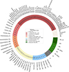 |
Figure 3 Clustering outcome after applying DBSCAN to a correlation matrix, resulting in eight distinct clusters of varying sizes indicated by their respective coloring, the numeric value added to each feature wedge represents the loading to the first principal component of the cluster that was subjected to principal component analysis (PCA). The feature-labels added to the legend were those being selected as key representatives of the respective cluster exposing the highest loading. Because of external validation reasons the A-rated sound pressure level was added to the list. |
2.4.3 Clustering procedure
A hierarchical clustering procedure was employed to group the average diurnal cycles, using the Ward method as the linkage criterion to minimize variance within clusters. That algorithm was contained in the python library SciPy (scipy.cluster.hierarchy.linkage [35]). To determine the clusters, the maxclust criterion algorithm was applied. This method identifies a minimum threshold (m) such that the cophenetic distance (the height of the dendrogram) between any two original observations within the same flat cluster does not exceed m. The algorithm also ensures that no more than t flat clusters are formed. For this analysis, nine clusters were selected, corresponding to the total number of land use type categories. To evaluate the clusters in relation to land use, respective land use types were integrated to the cluster dataframe and treated as the “true" cluster labels.
The Adjusted Rand Index (ARI) was selected as an external validity index to evaluate the performance of the clustering [36, 37], which is our approach to assessing how well the respective indices distinguish the land use types of the locations. The ARI algorithm measures the similarity between two sets of clusters, where one is designated as the ground truth. Importantly, it disregards permutations in cluster labeling. To calculate this metric, the two cluster sets are transformed into a contingency table that aggregates all possible pair of points belonging to the same cluster. The table is then used to break down the correct and incorrect assignments. In the subsequent step, the probabilities of specific combinations occurring by chance are accounted for. The ARI quantifies clustering performance on a scale ranging from −0.5 (highly discordant) to 1 (perfect alignment) [38]. While the metric provides a robust evaluation, we had to keep in mind that it could be less informative for smaller clusters in data sets with unbalanced cluster sizes, as the agreement for these clusters may be underrepresented [36].
3 Results
3.1 Dimensionality reduction
The best fit to the correlation clustering using DBSCAN was with 8 clusters and 8 noise points (silhouette score = 0.39, see Fig. 3). The first and most prominent cluster (with the highest number of indices) mainly contains indices related to sound volume, while the second is composed of kurtosis indices. The third cluster includes sharpness indices with loudness weighting (Aures method), and in the fourth group, spectral and roughness-related indices as well as also the ecoacoustic NDSI fall into this category. Clusters five comprise fluctuation strength indices and the Acoustic Complexity Index, respectively, whereas cluster six is represented by spectral entropy (Hf) and time/spectral entropy (H). The seventh cluster comprises the Acoustic Diversity Index as well as the Acoustic Evenness Index. The eighth cluster is defined by the Bioacoustic Index (in its two forms). Indices that did not cluster include Link Density, time-domain entropy (Ht), spectral balance (L(C) e q − L(A) e q ), Acoustic Richness (AR), the max-values of both of the sharpness indices, Number of Peaks (NP) and the Amplitude Index (M). Based on their loadings on their first principal component, the one that exposed the highest amount of explained variances (wedges of Fig. 3), we selected representative indices for each cluster. For a comprehensive overview of the PCA results, please refer to the supplementary material (Appendix B.2). All decisions were based on the highest loading value, besides the A-weighted sound pressure level (with a 1s time-weighting) as it played an important role in approaching the articulated research questions. For the first cluster, the root mean square aggregated loudness index (ISO 532-1 method – rms) was chosen as the representative index. In the second cluster, mean values of kurtosis exhibited the highest loading, making them the representative index for this dimension. Similarly, in the third cluster, rms-values had the highest loading, with sharpnessaures_rms as selected index. However, the total number of indices contributing to this component was lower compared to the first dimension. For the forth cluster, sharpnessdin_mean was selected as the representative index. In the fifth cluster, fluctuation_mean, a time-domain index, was identified with its mean showing the highest loading. The sixth cluster was represented by an ecoacoustic feature H, which is a product of frequency and time-domain elicited entropy, presumably highlighting its combined focus on both temporal and spectral information. In the seventh cluster, the representative index was the Acoustic Diversity Index, an ecoacoustic measure that captures variations in the spectral domain. Finally, the eighth cluster was represented by the Bioacoustic Index, which measures energy components within the spectral band ranging from 2 to 8 kHz, providing insight into specific spectral energy distributions. In addition, in the following analysis, seven indices identified as noise points (Fig. 3) are considered.
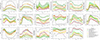 |
Figure 4 Diurnal plots of the main representatives, stratified by land use type, plotted with the 95% confidence interval and total amount of devices that fall into each land use category, ADI = Acoustic Diversity Index, BIO = Bioacoustic Index, H = Entropy, NP = Number of peaks, M = Amplitude index, AR = Acoustic richness, Ht = Temporal entropy. |
3.2 Diurnal cycles
Figure 4 shows the time of day averages of the selected main representatives. The data is stratified by LUT, which were not uniformly distributed (not every category occurs equally often). Although most indices demonstrate plausible low value ranges, kurtosis stands out with significant outliers, resulting in a large confidence interval. This is less evident, especially for loudness-related features. Despite being monitored with four devices, residential streets show a remarkable low inner variability, underscoring the uniformity of their sound environment. Across all plots, a clear distinction between day and night periods is evident, emphasizing the temporal dynamics of urban and peri-urban AEs.
Loudness-related indices (loudnessiso_rms and levela_eq_1) are most pronounced on main streets, and exhibit both high values and low intra-variability. In addition, there are peaks visible with notable and consistent difference compared to other land use types. Commercial and residential streets showed comparable loudness values although residential streets exhibited a distinctive peak at midday (12 PM). The A-weighted sound pressure level plot, however, does not reveal variations, compared with the other loudness index. Kurtosis emerges as a index with idiosyncrasies, as it shows distinctive patterns compared to the other indices, with urban forests ranking highest, albeit with considerable variability, while commercial areas rank lowest and show minimal day-night differences. Sharpness (Aures) mean values reveal significant differences between areas: urban forests exhibit the highest values, particularly at night, whereas commercial areas show consistently low values with almost no temporal variation. Main streets show lower sharpness at night than during the day. Peaks are visible in urban forests early in the morning (5 AM) and evening (8 PM), as well as similar but less pronounced increases observed in green spaces and residential areas.
A comparable trend is noted for mean sharpness values based on the DIN 45692 method. However, unlike the Aures method, residential streets do not experience an increase in sharpness during the day, highlighting the influence of loudness weighting in the Aures approach. Furthermore, differences between day and night periods are more distinctly recognizable in the DIN 45692 method. ADI values are highest in urban forests, with greater values observed at night. Main streets, on the other hand, show higher ADI values during the daytime, often surpassing even those recorded in urban forests. The playground area exhibited the lowest ADI values, with local peaks occurring in the morning hours. Agricultural land covers a broader range of ADI values, indicating variability in acoustic diversity depending on time and context. The Bioacoustic Index (BIO) is highest on main streets, apparently reflecting the dominance of anthropogenic and traffic-related sound sources, whereas urban forests display significant day-night differences, with higher values typically recorded during the day. In commercial areas, daytime differences in BIO-values are less pronounced, suggesting a more consistent AE throughout the day. In small gardens, BIO values tend to increase later in the day, reflecting an afternoon increase in acoustic activity. Entropy (H) values are consistently highest in urban forests and lowest in commercial areas, highlighting the greater variety of acoustic activity present in natural environments compared to the relatively homogeneous AE of commercial zones. Across all locations, entropy values dropped noticeably during midday, likely due to reduced overall activity during this period. Low-frequency content (L(C) e q − L(A) e q ) is most prominent in urban agricultural areas and is least pronounced on main streets. A notable drop in low-frequency content was observed across most sites in the early morning hours (around 5 AM), with values gradually building up again toward midday, reflecting diurnal changes in sound sources, such as the onset of vehicular activity. The comparison of sharpness indices – Aures (max) and DIN45692 (max) – reveals distinct patterns influenced by the incorporation of loudness weighting. Main streets exhibit the highest sharpness values when loudness is accounted for (Aures method), highlighting the dominance of high-energy, sharp sound sources in these environments. Day-night differences in sharpness are less pronounced across sites, although sharpness DIN (max) rose earlier in residential areas, potentially indicating the presence of different bird species active at dawn. Additionally, residential areas show a local sharpness peak at 4 PM, possibly reflecting a combination of human and natural sound events during this period. The Number of Peaks (NP) metric is highest at playgrounds and lowest on main streets, with a significant margin separating main streets from other land use types. This pattern is almost inverse to that observed for loudness-related variables, indicating a distinct relationship between NP and overall sound energy. The M metric exhibits the highest values in commercial areas, highlighting their consistently steady sound environment. Prominent peaks in M are observed at residential streets (2 PM), main streets (3 PM), and urban forests (9 AM), indicating temporal variations in sound activity across these land use types. Link Density is most pronounced on residential streets and lowest in urban forests, showing a clear stratification among land use types, with a notably high upper offset at main streets. A significant dip in Link Density is observed on both residential and main streets between 2:00 AM and 5:30 AM. Similar periodic patterns are evident across all other LUTs, with generally low activity levels at night. Regarding temporal variability, green areas exhibited the highest values of H t (temporal entropy), indicating greater variability in their AE, while gray urban areas showed the lowest values, with a pronounced local minimum around 5 PM. While all LUTs displayed a moderate drop in H t during this time, the decrease was most pronounced at the playground, whereas the main street values experience a rise during the same period. The Acoustic Richness (AR) metric is notably high in commercial areas, closely followed by forest areas. Peaks in AR are consistently observed at 6 AM across nearly all locations, with the most pronounced increases occurring in green areas, presumably highlighting the morning activity of both natural and anthropogenic sound sources.
3.3 Ward clustering
When examining ARI values in detail (see Fig. 5), a general low clustering quality becomes evident. While no single index fully represents the ground truth, four indices stand out with higher values. For example, fluctuation_mean yielded results that appeared random, whereas sharpnessaures_max consistently ranked as the most accurate index. Sharpnessdin_max, the non-loudness-weighted version of sharpness, received considerably lower scores compared to the Aures method, further emphasizing the influence of weighting methodologies on this metric’s performance. Link Density presents itself as the second-best index, though with lower values than the best predictor. Additionally, BIO and M indices perform at a comparable level, both achieving relatively high scores and marking a clear gap to the remaining indices.
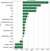 |
Figure 5 The Ward cluster labels of each device were compared with the corresponding land use type (taken from Tab. 1). The similarity between these two categories is quantified using the ARI (as described in Sect. 2.4.3), which is specified for each acoustic index. |
Beyond these findings, no single feature category (e.g., FCM-based, ecoacoustic, psychoacoustic, or SPL-aligned metrics) emerged as the dominant predictor of land use types. Instead, the top four indices were drawn from all categories, highlighting a distributed contribution across the calculated indices.
4 Discussion
This study addressed two core research questions related to the application of acoustic indices in urban environments. First, we examined whether acoustic indices provide additional information about the acoustic environment beyond traditional noise metrics such as L(A)eq. The findings clearly indicate that they do: acoustic indices demonstrate internal variability, highlight repetitive or periodic patterns, and demonstrate sensitivity to land use typologies, characteristics that SPL-based approaches tend to overlook. Second, we explored which acoustic indices convey similar or overlapping information. Our analysis revealed notable overlaps between ecological and psychoacoustic indices, particularly among those emphasizing peak or higher amplitude events. This insight contributes to the methodological refinement of future studies by helping to reduce redundancy in index selection. Collectively, the produced results merit further critical examination, focusing on three key aspects closely aligned with the research questions:
-
The Dataset Fingerprint: This section addresses the shared information discernible in the averaged data and explores its implications for understanding the overall structure and dimensionality of the dataset.
-
A Colorful Mosaic of the Acoustic Environment: The second focal point involves an interpretation of diurnal patterns within urban contexts, providing insight into the temporal dynamics of acoustic environments and their variability at different times of the day.
-
Land Use Type Clustering Fit: Finally, this section evaluates the functionality and suitability of the identified features, with particular attention to their role in distinguishing land use types.
4.1 The datasets fingerprint
The correlation analysis of the dataset reveals patterns consistent with findings of previous studies conducted in diverse contexts, including data with high spatial resolution [29], random 3D (ambisonic) audio samples [39], and binaural soundwalk recordings [26].
Across these studies, a consistent conclusion emerges regarding the first principal dimension: a group of loudness-related indices, that primarily capture sound volume, which also forms the most significant and cohesive block within our dataset. These parameters exhibit high internal consistency and are the dominant contributors in clustering analyses, characterized by low within-cluster variability. Psychoacoustic Annoyance is also included in this block, suggesting that its loudness weighting may be disproportionately emphasized for longitudinal analyses. To the authors’ knowledge, Psychoacoustic Annoyance (as defined by [15]) has not been previously calculated for longitudinal datasets, leaving limited opportunities for comparative evaluation.
The second major feature block encompasses spectral indices that capture frequency-related characteristics and integrate a combination of spectral and temporal features. This cluster highlights notable correlations between psychoacoustic parameters, such as sharpness and ecoacoustic indices like NDSI. This correlation is likely due to both measures being sensitive to high-frequency content, a phenomenon previously observed in related studies[29, 40]. Furthermore, Sharpness demonstrates strong correlations with Roughness within this dataset, which can likely be attributed to the repeated occurrence of specific sound sources characterized by rapid modulations in the high-frequency range.
Consistent with previous findings [29, 39], a distinct cluster related to slow modulation features was identified. Within this cluster, psychoacoustic indices like Fluctuation Strength display strong similarities with ecoacoustic indices, such as ACI. This correlation likely arises because both algorithms respond to periodic changes in the time-domain. ACI, for example, was specifically developed to detect irregular biophonic activity.
Kurtosis, on the contrary, forms a separate and highly distinct cluster, characterized by high internal variability and demonstrating notable inconsistency in behavior. Similarly, maximum sharpness indices diverge from other measures, but with considerably smaller confidence intervals underscoring their utility in longitudinal analyses.
Notably, the majority of ecoacoustic indices do not exhibit significant correlations with the primary clusters, highlighting their independence and value as complementary metrics to typical loudness and spectral indices. At this stage we can state that the structured interplay among various acoustic dimensions reinforce the potential of different acoustic indices to offer valuable insights into AEs.
4.2 Diurnal cycles as colorful mosaic of the acoustic environment
The use of time of day averaged value diagrams proves to be an effective and insightful method to represent the AE within urban areas. These visualizations reveal patterns that are both intuitive and, at times, less expected, offering a more advanced understanding of urban AE. One prominent observation is the periodic nature of certain acoustic indices, such as loudness indices that probably caused by the traffic volumes. These patterns are most pronounced on major roadways, emphasizing the dominant influence of vehicular noise on the urban AE. Nevertheless, variation in these values could as well be an indication of different road modalities such as intersections, highways, speed limits or commuting behavior, which could be investigated in future studies. Despite this well-known relationship, several other indices exhibit idiosyncratic patterns. Some align with expectations, while others appear counterintuitive. For instance, the Bioacoustic Index, which is typically associated with natural acoustic environments, reaches its highest values along main streets. This counterintuitive finding, already discussed in the literature [21], highlights that in urban contexts, the notion of highlighting activities in higher frequency bands, is not automatically linked to biophonic activity. Mechanical sounds occupy the full frequency spectrum, complicating straightforward interpretations of this particular ecoacoustic index.
Similarly, the ADI has also produced unexpected results. Prior studies have shown that ADI correlates negatively with human speech and positively with vehicle noise [41]. In our data, the forest site, where acoustic diversity would typically be expected to peak, actually exhibited higher ADI values during periods when biophonic activity should be more pronounced, suggesting a mismatch between index output and ecological expectation.
An unexpected pattern emerges when analyzing low-frequency prominence, measured as the difference between C-weighted and A-weighted sound pressure levels (L(C)eq − L(A)eq). Given that road traffic is the most prominent low-frequency source in populated areas, it would be reasonable to expect the highest values in locations with significant traffic presence. However, in this study, the highest values were observed in agricultural areas, where traffic noise is typically less dominant. This discrepancy suggests that additional factors influence the propagation and presence of low-frequency content. One potential explanation is the role of air absorption that counteracts the expected decrease in low-frequency prominence with increasing distance from major roads. The data also reveal distinct variations in commuting patterns and traffic composition, with traffic volumes peaking at specific times, such as early evening, and decreasing by midday. While these temporal variations are evident, more research is required to fully understand the mechanisms underlying this distribution.
The analysis of prominent peaks in the averaged acoustic data suggests that site-specific sounds are key contributors to the acoustic identity of urban and peri-urban environments. These distinctive patterns become more evident when examining time-specific or modulation-dependent parameters (Fluctuation Strength or M), highlighting the advantage of long-term acoustic monitoring. Unlike single-point measurements, which capture only a snapshot of the AE, automatized measurement periods reveal patterns and peculiarities that are otherwise difficult to discover.
4.3 Land use type clustering fit
Land use types were chosen as the ground truth for their ability to encapsulate the physical and functional characteristics of the built environment, which affect the AE. This classification should provide a structured framework for assessing how different acoustic indices capture the complexity and variability of the AE across diverse spatial contexts.
We employed a hierarchical clustering approach, a well-established method in the field, using Ward’s linkage criterion, which has proven effective in previous studies for forming meaningful clusters. These clusters were intended to reflect the underlying land-use patterns associated with the recording locations. Importantly, our primary objective was not to optimize predictive performance or to determine the most accurate method for land-use classification. Instead, our focus was on evaluating the responsiveness and suitability of a selected set of acoustic indices in capturing variations across different urban settings. For this reason, we did not refine the clustering procedure further or test multiple linkage methods extensively, as doing so might have risked overfitting the data and diverted attention from our core research aim.
The ARI emerged as a reliable clustering metric in the comparison of clustering procedures, as supported by existing literature. However, in this study, ARI produced relatively low scores, likely due to the challenging nature of the target classification: distinguishing among a large number (9) of closely related land use categories. Despite these challenges, the findings identified a subset of acoustic indices as predictors of land use categories.
Indices such as Sharpness Aures (max), Link Density, the Bioacoustic Index, and the median Amplitude Index (M) demonstrated considerable predictive utility, likely due to their strong correlations with dominant urban sound sources, including road traffic and human activity. In the case of Sharpness Aures, maximum values emerged as the most effective aggregation method. This outcome is expected, as the maximum values accentuate individual acoustic events, which often serve as defining characteristics of urban AE. By emphasizing peak occurrences, these metrics provide quantifiable insights into the influence of distinct sound events on the overall AE, which is probably linked to land use patterns.
The strong performance of the M index is particularly noteworthy, as it contrasts with the relatively poor predictive capacity of other dynamic features that capture the temporal evolution of sound events – such as Fluctuation Strength, Kurtosis, and Ht. These time-domain indices, which highlight impulsive events or slow signal modulations, appear unsuitable for this context. This discrepancy may be attributed to the dominance of long-term measurements, where transient or modulated events do not stand out.
In particular, loudness measures underperformed, probably because they fail to adequately emphasize the unique characteristics of individual sound sources that mark the specific land use. These findings suggest that site-specific acoustic characteristics are more effectively represented by fragments of the frequency spectrum, with maximum values as prioritized metric to capture central tendencies across a value series.
4.4 Limitations
Although the results demonstrate robustness and external validity, the spatial resolution of the data, limited to 23 monitoring stations, is insufficient for comprehensive city-wide acoustic evaluations. Future investigations should prioritize the deployment of a higher density of passive acoustic monitoring systems, particularly when examining extended temporal frameworks.
Our study cannot fully resolve what certain indices specifically represent in urban settings when applied in a time-series analysis. Although our findings suggest that some ecoacoustic and psychoacoustic indices may capture general tendencies linked to land-use types, they do not provide precise insights into specific sound sources or biological activity and it cannot be explained why indices such as Sharpness show particular patterns. More research, especially through microscale investigations or controlled laboratory/listening experiments, is needed to clarify the ecological significance of these metrics in urban contexts.
Moreover, inherent biases associated with PAM systems, as discussed in [42], necessitate the consideration of equalization filter curves in future studies to address potential discrepancies in data collection and analysis. Additionally, the computation of psychoacoustic parameters requires careful evaluation due to immanent challenges. These calculations are computationally intensive, require significant energy resources, and incur high operational costs.
5 Conclusion
The purpose of this study was to assess whether incorporating a curated array of acoustic metrics improves the characterization of acoustic environments beyond the typical noise measures. By expanding the analytical monitoring framework with additional metrics, the research sought to identify a set of indicators that offer a more nuanced understanding of the complexity of AEs. Additionally, it examined whether specific acoustic parameters exhibit numerical overlap and demonstrate consistency concerning the land use types associated with acoustic monitoring stations.
The findings underscore the limitations of traditional loudness-based measures and highlight the significance of frequency-specific and metrics that weight higher values in characterizing the AE – particularly the predictive strength of Sharpness Aures (max), Link Density, Bioacoustic Index and Amplitude Index for distinguishing land use types.
Nonetheless these results suggest that an expanded set of indices not only refines the analytical tools available to researchers but guides towards actionable insights for urban planners and designers.
N5 is the 95th percentile of loudness; the reverse designation is a convention in psychoacoustics. In this publication, we do not follow this convention, and in the following, P95 is referred to as the higher value.
Funding
This study was supported by the HEAD Genuit Foundation through a grant agreement (P-21/02-W).
Conflicts of interest
The authors declare no conflict of interest.
Data availability statement
Data are available on request from the authors.
Author contribution statement
Moritz Schuck: Writing – original draft, Visualization,Validation, Software, Methodology, Investigation, Formal analysis, Data curation, Conceptualization. Timo Haselhoff: Writing – review & editing, Validation, Methodology, Software, Formal analysis, Data curation. Bryce T. Lawrence: Writing – review & editing, Data curation, Software. Susanne Moebus: Writing – review & editing, Validation, Supervision, Resources, Project administration, Funding acquisition, Conceptualization. André Fiebig: Writing – review & editing, Supervision, Resources, Project administration, Funding acquisition.
Supplementary material
Appendix A1.1: Statistics per devices.
Appendix A1.2: Statistics per land use type.
Appendix A1.3: Diurnals per land use type and device.
Appendix B1.1: Correlation maps including all indices as heatmap.
Appendix B1.2: Correlation matrix in a spreadsheet.
Appendix B2: Principal component analysis loadings.
Appendix C1: Clustermaps of each acoustic index.
Access Supplementary MaterialReferences
- J. Kang, F. Aletta, E. Margaritis, M. Yang: A model for implementing soundscape maps in smart cities. Noise Mapping 5 (2018) 46–59. https://10.1515/noise-2018-0004. [Google Scholar]
- EEA: Environmental noise in Europe – 2020. Technical Reprot, 2020. Available at https://www.eea.europa.eu/en/analysis/publications/environmental-noise-in-europe (visited on01/24/2025). [Google Scholar]
- D. Espejo, V. Vargas, R. Viveros-Munoz, F.A. Labra, P. Huijse, V. Poblete: Short-time acoustic indices formonitoring urban-natural environments using artificial neural networks. Ecological Indicators 160 (2024) 111775. https://doi.org/10.1016/j.ecolind.2024.111775. [Google Scholar]
- EEA: Environmental noise in Europe 2025. Technical report, 2025. Available at https://www.eea.europa.eu/en/analysis/publications/environmental-noise-in-europe-2025 (visited on 11/07/2025). [Google Scholar]
- J. Wang, C. Li, Y. Lin, C. Weng, Y. Jiao: Smart soundscape sensing: A low-cost and integrated sensing system for urbansoundscape ecology research. Environmental Technology & Innovation 29 (2023) 102965. https://doi.org/10.1016/j.eti.2022.102965. [Google Scholar]
- A. Can, P. Audubert, P. Aumond, E. Geisler, C. Guiu, T. Lorino, E. Rossa: Framework for urban sound assessment at the city scale based on citizen action,with the smartphone application NoiseCapture as alever for participation. Noise Mapping 10 (2023) 20220166. https://10.1515/noise-2022-0166. [Google Scholar]
- C. Tarlao, F. Leclerc, J. Brochu, C. Guastavino : Current approaches toplanning (with) sound. Science of The TotalEnvironment 931 (2024) 172826. https://doi.org/10.1016/j.scitotenv.2024.172826. [Google Scholar]
- J. Alvarsson, S. Wiens, M. Nilsson: Stress recovery during exposure to nature soundand environmental noise. International Journal of Environmental Research and Public Health 7 (2010) 1036–1046. https://doi.org/10.3390/ijerph7031036. [CrossRef] [PubMed] [Google Scholar]
- S. Zielinski, F. Rumsey, S. Bech: On some biases encountered in modern audio quality listening tests – a review. Journal of the Audio Engineering Society 56 (2008) 427–451. [Google Scholar]
- L.S.M. Sugai, T.S.F. Silva, J.W. Ribeiro Jr., D. Llusia: Terrestrial passive acoustic monitoring: review and perspectives. BioScience 69 (2018) 15–25. https://doi.org/10.1093/biosci/biy147. [Google Scholar]
- O. Metcalf, C. Abrahams, B. Ashington, E. Baker, T. Bradfer-Lawrence, E. Browning, J. Carruthers-Jones, J. Darby, J. Dick, A. Eldridge, D. Elliott, B. Heath, P. Howden-Leach, A. Johnston, A. Lees, C. Meyer, U. Ruiz Arana, S. Smyth: Good practice guidelines for long-term ecoacoustic monitoring in the UK. Technical report, 2023. [Google Scholar]
- D. Bonet-Solà, E. Vidaña-Vila, R.M. Alsina-Pagès: Prediction of the acoustic comfort of a dwelling based on automatic sound event detection. Noise Mapping 10 (2023) 20220177. https://doi.org/10.1515/noise-2022-0177. [Google Scholar]
- R. Ventura, V. Mallet, V. Issarny: Assimilation of mobile phone measurements for noise mapping of a neighborhood. Journal of the Acoustical Society of America 144 (2018) 1279–1292. https://doi.org/10.1121/1.5052173. [Google Scholar]
- L. Brocolini, C. Lavandier, M. Quoy, C. Ribeiro: Measurements of acoustic environments for urban soundscapes: choice of homogeneous periods, optimization of durations, and selection of indicators. Journal of the Acoustical Society of America 134 (2013) 813–821. https://doi.org/10.1121/1.4807809. [Google Scholar]
- E. Zwicker, H. Fastl: Psychoacoustics: facts and models, 2nd updated edn. Springer, Berlin, New York, 1999. ISBN: 978-3-540-65063-8. [Google Scholar]
- M.S. Engel, A. Fiebig, C. Pfaffenbach, J. Fels: A review of the use of psychoacoustic indicators on soundscape studies. Current Pollution Reports 7, 3 (2021), 359–378. https://doi.org/10.1007/s40726-021-00197-1. [CrossRef] [Google Scholar]
- C. Lavandier, B. Defreville: The contribution of sound source characteristics in the assessment of urban soundscapes. Acta Acustica United with Acustica 92 (2006) 912–921. [Google Scholar]
- M. Yang, J. Kang: Psychoacoustical evaluation of natural and urban sounds in soundscapes. Journal of the Acoustical Society of America 134, 1 (2013) 840–851. https://doi.org/10.1121/1.4807800. [Google Scholar]
- M. Nilsson, B. Berglund: Soundscape quality in suburban green areas and city parks. Acta Acustica united with Acustica 92 (2006) 903–911. [Google Scholar]
- B.T. Lawrence, J. Hornberg, T. Haselhoff, R. Sutcliffe, S. Ahmed, S. Moebus, D. Gruehn: A widened array of metrics (WAM) approach to characterize the urban acoustic environment; a case comparison of urban mixed-use and forest. Applied Acoustics 185 (2022) 108387. https://doi.org/10.1016/j.apacoust.2021.108387. [Google Scholar]
- T. Haselhoff, B. Lawrence, J. Hornberg, S. Ahmed, R. Sutcliffe, D. Gruehn, S. Moebus: The acoustic quality and health in urban environments (SALVE) project: study design, rationale and methodology. Applied Acoustics 188 (2022) 108538. https://doi.org/10.1016/j.apacoust.2021.108538. [Google Scholar]
- T. Haselhoff, T. Braun, J. Hornberg, B.T. Lawrence, S. Ahmed, D. Gruehn, S. Moebus: Analysing interlinked frequency dynamics of the urban acoustic environment. International Journal of Environmental Research and Public Health 19 (2022) 15014. https://doi.org/10.3390/ijerph192215014. [Google Scholar]
- J. Sueur: Sound analysis and Synthesis withR. Use R! Springer International Publishing, Cham, 2018. ISBN: 978-3-319-77645-3 978-3-319-77647-7. https://doi.org/10.1007/978-3-319-77647-7. [Google Scholar]
- T. Haselhoff, T. Braun, A. Fiebig, J. Hornberg, B.T. Lawrence, N. Marwan, S. Moebus: Complex networks for analyzing the urban acoustic environment. Ecological Informatics 78 (2023) 102326. https://doi.org/10.1016/j.ecoinf.2023.102326. [Google Scholar]
- W. Aures: Berechnungsverfahren für den sensorischen Wohlklang beliebiger Schallsignale. Acustica 59 (1985) 130–141. [Google Scholar]
- M. Rychtarikova, G. Vermeir: Soundscape categorization on the basis ofobjective acoustical parameters. Applied Acoustics 74 (2013) 240–247. https://doi.org/10.1016/j.apacoust.2011.01.004. [Google Scholar]
- C. Asensio, P. Aumond, A. Can, L. Gascó, P. Lercher, J.-M. Wunderli, C. Lavandier, G. de Arcas, C. Ribeiro, P. Muñoz, G. Licitra: A taxonomy proposal for the assessment of the changes in soundscape resulting from the COVID-19 lockdown. International Journal of Environmental Researchand Public Health 17, 12 (2020) 4205. https://doi.org/10.3390/ijerph17124205. [Google Scholar]
- Josef Schlittenlacher et al. Overall loudness of short time-varying sounds. In: Davy J, Ed. Proceedings – 43rd International Congress and Exposition on Noise Control Engineering (Internoise 2014), Melbourne, 16–19 November, Australian Acoustical Society (AAS), Melbourne, Australia, 2015. [Google Scholar]
- T. Haselhoff, M. Schuck, B.T. Lawrence, A. Fiebig, S. Moebus: Characterizing acoustic dimensions of health-related urban greenspace. Ecological Indicators 166 (2024) 112547. https://doi.org/10.1016/j.ecolind.2024.112547. [Google Scholar]
- W. Qiu, W. Murphy, A. Suter: Kurtosis: a new tool for noise analysis. Acoustics Today 16 (2020) 39–47. https://doi.org/10.1121/AT.2020.16.4.39. [Google Scholar]
- Jonas Hornberg et al: Impact of the COVID-19 lockdown measures on noise levels in urban areas-A pre/during comparison of long-term sound pressure measurements in the Ruhr Area, Germany. International Journal of Environmental Research and Public Health 18, 9 (2021) 4653. https://doi.org/10.3390/ijerph18094653. [Google Scholar]
- E. Kreyszig: Advanced engineering mathematics, 4th edn. John Wiley and Sons Ltd, New York, 1979. ISBN: 978-0-471-04271-6. [Google Scholar]
- M. Ester, H.-P. Kriegel, J. Sander, X. Xu: A density-based algorithm for discovering clusters in large spatial databases with noise. Knowledge Discovery and Data Mining, 1996. Available at https://api.semanticscholar.org/CorpusID:355163. [Google Scholar]
- P.J. Rousseeuw: Silhouettes: a graphical aid to the interpretation and validation of cluster analysis. Journal of Computational and Applied Mathematics 20 (1987), 53–65. https://doi.org/10.1016/0377-0427(87)90125-7. [CrossRef] [Google Scholar]
- scipy.cluster.hierarchy.linkage. Available at https://docs.scipy.org/doc/scipy/reference/generated/scipy.cluster.hierarchy.linkage.html#scipy.cluster.hierarchy.linkage. [Google Scholar]
- M.J. Warrens, H. Van Der Hoef: Understanding the adjusted rand index and other partition comparison indices based on counting object Pairs. Journal of Classification 39, 3 (2022) 487–509. https://doi.org/10.1007/s00357-022-09413-z. [Google Scholar]
- D. Steinley: Properties of the Hubert-Arabie adjusted Rand index. Psychological Methods 9, 3 (2004) 386–396. https://doi.org/10.1037/1082-989X.9.3.386. [Google Scholar]
- J.E. Chacón, A.I Rastrojo: Minimum adjusted Rand index for two clusterings of a given size. Advances in Data Analysis and Classification 17 (2023) 125–133. https://doi.org/10.1007/s11634-022-00491-w. [Google Scholar]
- J. Bergner, J. Peissig: On the identification and assessment of underlying acoustic dimensions of soundscapes. Acta Acustica 6 (2022) 46. https://doi.org/10.1051/aacus/ 2022042. [CrossRef] [EDP Sciences] [Google Scholar]
- M.S. Engel, W. Davies, R.J. Young: Understanding natural sound sources in urban soundscapes through psychoacoustic and bioacoustic indicators. In: Fortschritte der Akustik-DAGA 2023, Hamburg, 2023. [Google Scholar]
- A.J. Fairbrass, P. Rennert, C. Williams, H. Titheridge, K.E. Jones: Biases of acoustic indices measuring biodiversity in urban areas. Ecological Indicators 83 (2017) 169–177. https://doi.org/10.1016/j.ecolind.2017.07.064. [Google Scholar]
- A. Potenza, V. Zaffaroni-Caorsi, R. Benocci, G. Guagliumi, J.M. Fouani, A. Bisceglie, G. Zambon: Biases in ecoacoustics analysis: a protocol to equalize audio recorders. Sensors 24 (2024) 4642. https://doi.org/10.3390/s24144642. [Google Scholar]
Cite this article as: Schuck M. Haselhoff T. Lawrence B.T. Moebus S. & Fiebig A. 2025. Advancing the characterization of urban acoustic environments through multimetric analysis. Acta Acustica, 9, 66. https://doi.org/10.1051/aacus/2025051.
All Tables
All Figures
|
Figure 1 Methods used and outcome produced to address the research questions, the numbers in the brackets indicate the dimensions of the data structure, the first two steps we took in order to understand numerical overlap of the predefined set of indices, later we used PCA to select non-arbitrary indices as cluster representatives. This set of uncorrelated indices was then checked regarding sensitivity and response to the land use type where the device was positioned through a statistical procedure that included common clustering methods and the calculation of a validation metric. |
| In the text | |
|
Figure 2 Overview of daily count of recordings for each device. The breaks between the dots represent a period of missing data, non-blue dots represent days with a total count of recordings < 50. |
| In the text | |
|
Figure 3 Clustering outcome after applying DBSCAN to a correlation matrix, resulting in eight distinct clusters of varying sizes indicated by their respective coloring, the numeric value added to each feature wedge represents the loading to the first principal component of the cluster that was subjected to principal component analysis (PCA). The feature-labels added to the legend were those being selected as key representatives of the respective cluster exposing the highest loading. Because of external validation reasons the A-rated sound pressure level was added to the list. |
| In the text | |
|
Figure 4 Diurnal plots of the main representatives, stratified by land use type, plotted with the 95% confidence interval and total amount of devices that fall into each land use category, ADI = Acoustic Diversity Index, BIO = Bioacoustic Index, H = Entropy, NP = Number of peaks, M = Amplitude index, AR = Acoustic richness, Ht = Temporal entropy. |
| In the text | |
|
Figure 5 The Ward cluster labels of each device were compared with the corresponding land use type (taken from Tab. 1). The similarity between these two categories is quantified using the ARI (as described in Sect. 2.4.3), which is specified for each acoustic index. |
| In the text | |
Current usage metrics show cumulative count of Article Views (full-text article views including HTML views, PDF and ePub downloads, according to the available data) and Abstracts Views on Vision4Press platform.
Data correspond to usage on the plateform after 2015. The current usage metrics is available 48-96 hours after online publication and is updated daily on week days.
Initial download of the metrics may take a while.