| Issue |
Acta Acust.
Volume 9, 2025
|
|
|---|---|---|
| Article Number | 76 | |
| Number of page(s) | 14 | |
| Section | Underwater Sound | |
| DOI | https://doi.org/10.1051/aacus/2025060 | |
| Published online | 09 December 2025 | |
Scientific Article
Finite element optimization and performance analysis of a multi-driven Tonpilz transducer
1
College of Ship and Ocean Engineering, Jiangsu University of Science and Technology, Zhenjiang, 212000, PR China
2
College of Ocean, Jiangsu University of Science and Technology, Zhenjiang, 212000, PR China
* Corresponding author: This email address is being protected from spambots. You need JavaScript enabled to view it.
; This email address is being protected from spambots. You need JavaScript enabled to view it.
Received:
12
April
2025
Accepted:
27
October
2025
Abstract
To improve broadband transmission performance of mid-frequency transducers, the finite element method was applied to optimize and analyze the performance of a multi-driven Tonpilz transducer, focusing on excitation methods and structural design. A multi-driven Tonpilz transducer with a radiating head containing concentric-ring cavities was proposed, in which multi-cavity design reduces effective mass and enhances bandwidth. The performance under three excitation methods was evaluated by comparing admittance curves in air and analyzing resonant modes, revealing the effects of excitation methods on electromechanical coupling and resonant peaks. Partial excitation was identified as the optimal approach. The impedance characteristics, vibrational modes, and acoustic directivity in water were further investigated. The effects of the mass block, radiating head containing concentric-ring cavities, and front cover on transmitting voltage response fluctuations were analyzed. After optimization, the transducer operates over 17 kHz–41 kHz, with a −3 dB bandwidth of 24 kHz and a maximum transmitting voltage response of 143.7 dB re 1 μPa/V @ 1 m, providing a foundation for applications in related fields.
Key words: Finite element method / Optimization design / Broadband / Tonpilz transducer / Transmitting voltage response
© The Author(s), Published by EDP Sciences, 2025
 This is an Open Access article distributed under the terms of the Creative Commons Attribution License (https://creativecommons.org/licenses/by/4.0), which permits unrestricted use, distribution, and reproduction in any medium, provided the original work is properly cited.
1 Introduction
Underwater acoustic transducers play a critical role in modern underwater systems due to their capability to generate and detect sound efficiently [1–4]. Expanding transducer bandwidth is essential for improving the performance of underwater acoustic systems. In applications such as marine monitoring and military reconnaissance, wideband transducers enable higher-rate underwater communication and multi-task operations [5–7]. Among various types of underwater transducers, the Tonpilz transducer is most commonly used, owing to its simple manufacturing process, compact size, and high output power [8–11]. However, traditional Tonpilz transducers are limited by their single-mode operating principle, relying only on longitudinal resonance modes, which constrains frequency band extension. This narrowband characteristic restricts both the information capacity of underwater communication and the target resolution of sonar systems, limiting the fulfillment of technical demands for broadband sound sources in modern marine engineering [12].
To address the critical challenge of improving broadband performance, current research focuses on three main aspects: excitation source optimization, structural optimization, and impedance matching, all of which are achieved using multimode transducers [13–16]. It has been shown that multiple excitation sources can effectively broaden the bandwidth of Tonpilz transducers. The dual-excitation transducer, proposed by Thompson, excites composite vibration modes and significantly expands the operating frequency range [17]. Building on this, J.L. Butler and S.C. Butler combined magnetostrictive materials with piezoelectric ceramics, and through the synergistic effects of these materials, successfully induced a dual-resonance phenomenon [18, 19]. Subsequently, Butler et al. introduced an unconventional excitation method that requires the excitation of only half of the piezoelectric stack to simultaneously activate the first three longitudinal vibration modes, thus providing a new approach for excitation technology innovation [20]. Regarding excitation source structural parameters, Zhang et al. confirmed that the size ratio between the intermediate mass block and the piezoelectric stack is critical to multimode coupling efficiency, offering guidance for parameter optimization [21]. Pyo et al. proposed anon-uniform piezoelectric ceramic stacking scheme that supports phase difference control and impedance matching [22]. Ji et al. further confirmed that a multi-driver stacking structure can activate continuous high-order longitudinal resonance modes, and the distributed excitation of the driving units can overcome the bandwidth limitations inherent in traditional single-mode coupling[23, 24]. Therefore, the selection of an appropriate excitation mode for the transducer is crucial.
In structural optimization, the radiating head structure has become a central focus in recent years. Its length and radiating area influence not only the excitation of flexural vibration modes but also significantly regulate the radiating quality factor [25]. Based on mechanical quality factor control theory, He et al. enhanced multimode coupling by introducing specific geometric features into the radiating head [26, 27]. Kim and Roh reported that the introduction of a hollow head mass in Tonpilz transducers led to a relative bandwidth of 130.7%, significantly outperforming traditional designs [28, 29]. A common feature of these optimization strategies is their ability to improve mode coupling and broaden bandwidth by modifying the radiating head’s geometric structure, highlighting the critical role of structural design in enhancing transducer performance. Regarding impedance matching, Ji et al. proposed a phononic crystal matching layer that improves bandwidth characteristics by suppressing transverse vibrations [30]. Additionally, the 3D printed gradient matching layer developed by Bian et al. achieved a 110% −3 dB bandwidth in experimental tests, providing new insights for high-frequency broadband transducer design [31]. The selection of matching layer materials and manufacturing precision is crucial, as poor matching leads to energy loss, and its performance stability may be affected in complex environments [32, 33].
The finite element method was applied to optimize and analyze the performance of a multi-driven Tonpilz transducer with a radiating head containing concentric-ring cavities. Effects of different excitation methods on transmitting voltage response were examined, and differences in admittance curves in air, as well as impedance characteristics, vibrational modes, and acoustic directivity in water, were analyzed. Finally, optimization of mass block, front cover, and radiating head containing concentric-ring cavities dimensions allowed adjustment of frequencies and amplitudes of resonant peaks in transmitting voltage response, resulting in enhanced transducer performance.
2 Structure of the multi-driven tonpilz transducer
The traditional Tonpilz transducer, shown in Figure 1, consists of a tail mass, a piezoelectric ceramic stack, a prestressed bolt, and a metal horn-shaped radiating head. The piezoelectric ceramic stack is composed of multiple piezoelectric ceramic layers with opposite polarities, which are mechanically connected in series and electrically in parallel. Adhesive is applied to the connecting surfaces during the manufacturing process to enhance the bonding strength between the components. The bandwidth of traditional Tonpilz transducers is typically narrow, limiting their suitability for wideband applications [34]. This limitation results from the high mechanical quality factor and the energy concentration associated with a single vibrational mode. Therefore, optimizing the bandwidth of these transducers requires addressing both factors.
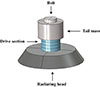 |
Figure 1. Traditional Tonpilz underwater acoustic transducer structure. |
The radiation resistance R r is expressed as
 (1)
(1)
where ρ is the medium’s density, c is the speed of sound in the medium, k is the wave number, and S is the radiating surface area of the transducer head [25]. Since the cavity structure primarily alters the internal volume without affecting the radiating surface area S, the radiation resistance R r can be considered unchanged.
The mechanical quality factor of the Tonpilz transducer can be expressed as
 (2)
(2)
where M h is the equivalent mass of the transducer head, and R r is the radiation resistance [29, 35].
A wide bandwidth is achieved by increasing vibrational mode frequencies, typically through adjusting the stiffness-to-mass ratio of the vibrating structure. However, the resulting frequency enhancement often increases the geometric thickness of the transducer head [28]. According to the formula, Q m is proportional to M h , which limits bandwidth optimization [36]. To address this, a controlled method is required to adjust the transducer head thickness without increasing its mass. This study proposes a cavity structure within the radiating head to reduce its mass, as shown in Figure 2. The radiating head comprises three concentric annular cavities. By adjusting the cavity dimensions, the mass can be controlled within a desired range, thereby providing greater flexibility for subsequent bandwidth optimization. Maintaining the head thickness ensures the preservation of the effective radiating surface area and structural rigidity, thereby facilitating the efficient excitation andinteraction of multiple vibrational modes [26–29]. In practical engineering applications, the radiating head and front cover are connected by a threaded connection based on mechanical fastening principles, as shown in Figure 3. In simulation models, this connection is often simplified to a rigid interface to improve computational efficiency.
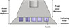 |
Figure 2. Schematic diagram of the head mass with cavity. |
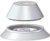 |
Figure 3. Schematic diagram of the connection between the radiating head and the front cover in practical applications. |
The structural schematic of the multi-driven Tonpilz transducer designed in this study, with a radiating head containing concentric-ring cavities, is illustrated in Figure 4. Concentric-ring cavities are integrated into the hard aluminum radiating head to enable multi-mode coupling and broaden the transducer bandwidth. The radiating head, front cover, and piezoelectric ceramic areconnected using a 45# steel bolt. Three brass mass blocks are added to adjust the overall frequency response characteristics. A 2:2:2 proportional configuration is applied to the piezoelectric ceramic Lead Zirconate Titanate-4 (PZT-4). The density ρ, Young’s modulus E, Poisson’s ratio ν of the transducer material, and the main dimensions of the transducer are provided in Tables 1 and 2. In practice, the metal electrode and adhesive layers, due to their minimal thickness, exert negligible influence on the transmitting voltage response of the underwater acoustic transducer. Furthermore, prestress is primarily applied in the design to ensure structural stability. Its impact on sound transmitting efficiency is minor and does not significantly affect broadband response optimization, thus it is omitted from the model [18].
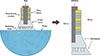 |
Figure 4. Schematic diagram of the multi-driven Tonpilz transducer with a radiating head containing concentric-ring cavities. |
Material parameters of the Tonpilz transducer.
Main dimensions of the Tonpilz transducer.
3 Finite element modeling
COMSOL Multiphysics can be used to develop frequency-domain models for analyzing harmonic excitation response problems involving single or multiple frequencies [37]. The simulation is configured with a maximum frequency of 60 kHz and a frequency step size of 100 Hz.
3.1 Boundary condition setup
Voltage boundary conditions play a crucial role in simulating hydroacoustic transducers, requiring proper excitation on the electrode surfaces of the piezoelectric ceramic components to accurately replicate their operational states. As shown in Figure 5, the six piezoelectric ceramic rings are polarized alternately, with three polarized in the +Z direction and the other three in the −Z direction. To simulate typical electrical excitation conditions, a voltage of 1 V is applied between the electrodes.
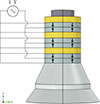 |
Figure 5. Schematic diagram of polarization directions and electrical connections of piezoelectric ceramic rings. |
To prevent sound reflection at the interface between the radiating head in the solid domain and other sound propagation media, the contact region must be defined as an acoustical-structural boundary. An external field computation area must also be established in the pressure acoustics model to accurately calculate the sound pressure distribution, with the acoustic radiation surface defined as the external field boundary. A Perfectly Matched Layer (PML) is employed to model the acoustic characteristics of an infinite water body, forming a closed domain. Scattered waves are absorbed upon reaching the PML, preventing interference with the scattered sound field in the space [38].
3.2 Mesh setup
Based on the characteristics of the model, a 2D axisymmetric module is employed for simulation. To ensure the precision of sound pressure wave analysis in the aquatic environment, the maximum grid size must satisfy the following condition
 (3)
(3)
where Vw = 1500 m/s is the sound speed in water and fmax = 60 kHz is the maximum frequency of the transducer [39].
Free triangular elements discretize the solid domain of the transducer, with the grid size set to Lmax to ensure a smooth mesh transition. To meet PML accuracy requirements, an eight-layer structured mesh is employed. A boundary layer mesh is applied within the inner water domain near the external field boundary, with its thickness set to one-fourth of Lmax. This layer ensures a smooth transition between the internal free triangular mesh and the external structured mesh, improving the accuracy of external field calculations. The finite element mesh model is shown in Figure 6.
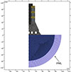 |
Figure 6. Transducer finite element mesh. |
4 Finite element analysis
Transmitting Voltage Response (TVR) is defined as the ratio of the free-field sound pressure at 1 m from the equivalent acoustic center of a transducer on its acoustic axis to the input voltage [18]. The axial sound pressure at 1 m is extrapolated from the far field under the assumption of spherical divergence. TVR, expressed in dB re 1 μPa per volt, directly indicates transducer performance, and bandwidth optimization has become a consensus in underwater acoustic transducer research [12]. The transmitting voltage response in this study is calculated based on the axial far-field sound pressure amplitude, measured 1 m in front of the head mass, relative to 1 μPa/V.
The transmitting voltage response is determined using the following equation
 (4)
(4)
where pRMS is the root-mean-square sound pressure at a reference distance of 1 m, and VRMS is the root-mean-square voltage applied to the transducer [18].
4.1 Piezoelectric ceramic stack excitation methods analysis
The piezoelectric ceramic stacks play a critical role in transducer design. The excitation strategy of the stacks significantly influences the ability of the transducer to effectively excite various longitudinal resonant modes and achieve a smooth transmitting voltage response without significant dips [22, 24, 40, 41]. This paper discusses three excitation methods for the piezoelectric ceramic stacks: in-phase excitation, anti-phase excitation, and partial excitation as shown in Figure 7.
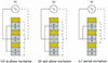 |
Figure 7. Different excitation methods of the piezoelectric ceramic stacks. (a) In-phase excitation. (b) Anti-phase excitation. (c) Partial excitation. |
Figure 8 shows the transmitting voltage response of the Tonpilz transducer under three excitation methods. The bandwidth and amplitude under anti-phase excitation are lower than those of the other two methods, with a distinct dip observed at 34.9 kHz. The in-phase and partial excitation responses exhibit similar overall shapes but opposite variation trends. Under in-phase excitation, the response amplitude first increases and then decreases, whereas partial excitation achieves higher performance in the mid- to high-frequency range. Within 19–45 kHz, both the number and magnitude of resonant peaks vary depending on the excitation method, and the dip caused by anti-phase excitation remains particularly evident.
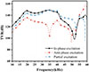 |
Figure 8. Transmitting voltage response under different excitation methods. |
Admittance serves as a key parameter for characterizing system resonance and revealing the mechanisms underlying variations in transmitting voltage response under different excitation methods [18]. To investigate the resonant behavior and energy conversion mechanisms of the Tonpilz transducer, its admittance characteristics in air were analyzed to remove the influence of water damping on resonance assessment. Figure 9 shows the admittance and corresponding resonant mode distributions of the transducer in air under different excitation methods, with a blue-to-red gradient representing increasing total displacement amplitude. Within the15–45 kHz frequency range, up to three resonant peaks are observed, corresponding to longitudinal vibration and flexural–longitudinal coupled vibration modes. Under in-phase and partial excitations, all three peaks are clearly present, with admittance under in-phase excitation being weaker than that under partial excitation. In contrast, anti-phase excitation reduces peak amplitude. As shown in Figure 9blued, the resonant peak at 34.6 kHz under anti-phase excitation is particularly inconspicuous, indicating poor mode excitation. The vibration mode at this frequency exhibits pronounced local compression at the piezoelectric ceramic, causing amplitude cancellation and energy loss, ultimately resulting in a very low transmitting voltage response. These observations further indicate that the excitation method regulates resonant mode activation by influencing the electromechanical couplingprocess of the transducer, consistent with the observed variations in transmitting voltage response. From a performance optimization perspective, activating more vibration modes is a key approach to broadening the operational frequency range; accordingly, partial excitation is employed to optimize transmission performance [42].
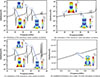 |
Figure 9. Admittance and resonant modes of the Tonpilz transducer in air under different excitation methods. (a) Admittance of the transducer under in-phase excitation. (b) Admittance of the transducer under anti-phase excitation. (c) Admittance of the transducer under partial excitation. (d) Amplified admittance curve under 34.6 kHz anti-phase excitation. |
4.2 Impedance characteristics analysis in water
The simulation results of the transducer conductance G and susceptance B in water are shown in Figure 10, which presents the admittance in water with the first four resonant frequencies occurring at 19.3 kHz, 34.9 kHz, 40.2 kHz, and 51.5 kHz. The first two peaks of G increase with frequency, while the subsequent peaks decrease. At the third resonant frequency, G reaches its maximum, representing the optimal operating frequency. In the underwater environment, the circuit is predominantly capacitive in most cases. At higher frequencies, the transducer vibrations become more complex, and the impact of the load on the radiating surface also becomes more intricate.
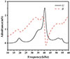 |
Figure 10. Transducer conductance-susceptance result. |
The impedance characteristic reveals that conductance and susceptance vary with frequency, directly reflecting impedance changes across the frequency range. However, electrical parameters alone cannot fully explain the vibration mechanisms, so modal vibration analysis is employed to reveal the vibration modes at each resonant frequency from a structural dynamicsperspective.
4.3 Vibration modal analysis
Figure 11 illustrates vibration modes of the transducer under water loading. At the first resonant frequency shown in Figure 11a, vibration is dominated by longitudinal vibration of the piezoelectric stack and the radiating head, enhancing axial acoustic wave radiation and improving radiation efficiency. At the second and third resonant frequencies shown in Figures 11b and 11c, nodal planes divide the transducer into multiple vibration regions, and the radiating head exhibits outward flexural vibration. Surface displacement concentrates in the circumferential regions, accompanied by longitudinal vibration of the piezoelectric stack, forming longitudinal–flexural coupled vibration. At the second resonant frequency, front cover and central region amplitude is extremely low, with downward flexural deformation observed on both sides of the center. At the third resonant frequency, vibration of the radiating head becomes more uniform, and the front cover exhibits larger amplitude. At the fourth resonant frequency shown in Figure 11d, vibration becomes more complex, with the radiating head cavity exhibiting longitudinal–radial coupled vibration and localized high-amplitude points in the front cover region.
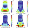 |
Figure 11. Vibration modes of the transducer under water loading. (a) First resonance – 19.3 kHz. (b) Second resonance – 34.9 kHz. (c) Third resonance – 40.2 kHz. (d) Fourth resonance – 51.5 kHz. |
4.4 Acoustic directivity analysis
The vibration modes significantly affect the acoustic radiation characteristics of the transducer. Therefore, a sound radiation analysis is essential to further elucidate the coupling mechanisms behind these characteristics. The −3 dB beamwidth is defined as the angular separation between the points where the main lobe response decreases by 3 dB from the peak value [18]. It is a key parameter for evaluating transducer directivity and can be directly calculated through the beamwidth setting in COMSOL.
Acoustic radiation analysis requires distinguishing between the far-field and near-field, primarily based on the propagation characteristics of sound waves, especially the calculation of the Rayleigh distance. The Rayleigh distance R defines the transition point between the near-field and far-field after sound waves are emitted by the transducer, and its formula is
 (5)
(5)
where D is the effective diameter of the transducer, and λ is the wavelength of the sound wave [18]. In the near-field (when the distance is less than the Rayleigh distance), beamwidth becomes complex due to interference effects on the sound pressure distribution, which depends on both distance and direction. In contrast, in the far-field, sound wave propagation tends to be a plane wave, and the sound pressure distribution stabilizes [43]. Therefore, this paper focuses on the study of far-fieldbeamwidth.
Simulations were conducted at a distance of 10 m from the radiating head (absolute far-field) and perpendicular to it. Figure 12 presents the radiation pattern of the transducer at its resonant frequency, with the units of the curves in the legend being dB. The far-field −3 dB beamwidths at 19.3 kHz, 34.9 kHz, 40.2 kHz, and 51.5 kHz were 60.57°, 30.31°, 101.81° and 80.08°, respectively. Flexural vibration occurs in the radiating head of the Tonpilz transducer at mid frequencies. The amplitude difference between the center and the outer periphery influences the energy radiation angle, leading to a significant variation in radiation angles at 34.9 kHz and 40.2 kHz. In contrast, the beamwidths at 19.3 kHz and 51.5 kHz fall between those of the two frequencies, reflecting axial radiation characteristics dominated by longitudinal vibration and energy dispersion caused by localized high-amplitude regions.
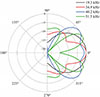 |
Figure 12. Radiation pattern of the transducer at different resonant frequencies. |
5 Transducer bandwidth optimization
Figure 13 presents the transmitting voltage response of the transducer. The results demonstrate that, within the frequency range of 18–40 kHz, the underwater Tonpilz transducer shows a relatively flat response curve. However, the fluctuation in transmitting voltage response exceeds 6 dB (peak-to-peak), failing to meet the design requirement for underwater communication, which specifies that TVR fluctuations should be controlled within 3 dB (peak-to-peak) in the 17–41 kHz range [7]. To achieve the desired bandwidth, optimization of the transducer’s structural dimensions is required. The analytical method employed in this study involves modifying specific parameters of one component while keeping all other parameters constant. This approach facilitates a deeper understanding of how independent variations in structural components improve transducer performance.
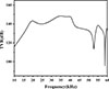 |
Figure 13. Transmitting voltage response before optimization. |
In the dimensional optimization analysis, the undisturbed parameter values are defined as the initial structural dimensions of the transducer, as shown in Table 2. The selection of the parameter variation range accounts for both manufacturing feasibility and design experience. For each structural parameter, adjustments are made in 1 mm steps, using the undisturbed values as a baseline. If, after a 1 mm step simulation, the change in transmitting voltage response is insignificant, a 2 mm step is applied. The step size is determined based on common precision levels in mechanical processing to ensure that parameter variations are feasible from an engineering perspective and can significantly influence transducer performance. If the analysis shows that the optimal value lies at the endpoint of the variation range, the influence of dimensional factors on transducer performance should be evaluated to determine if the endpoint value satisfies the design requirements. If further performance improvement necessitates exceeding the original range, the simulation should be extended by expanding the range to verify whether the optimal dimensional factor is constrained by the initial range or by physical limits.
As shown in Figure 14, mass block thickness has an effect on the transmitting voltage response. Within the 18–26 kHz range, increasing mass block thickness slightly reduces the transmitting voltage response. In the 26–38 kHz range, increasing thickness leads to an overall increase in transmitting voltage response. Beyond 38 kHz, the transmitting voltage response decreases more significantly with increasing thickness. From a vibration perspective, increased mass block thickness raises the total transducer mass, which inhibits vibration of the piezoelectric ceramics and affects overall performance. Therefore, mass block thickness should be controlled to prevent excessive bandwidth narrowing and responseinstability.
 |
Figure 14. Effect of mass block thickness on transmitting voltage response. (a) Front mass block. (b) Middle mass block. (c) Rear mass block. |
The front cover and radiating head work together to efficiently radiate and transmit sound waves. The schematic diagram of their dimensional optimization is shown in Figure 15.
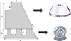 |
Figure 15. 2D symmetric geometry and 3D modeling of the front cover and radiating head. |
The simulation results are shown in Figure 16, where the outer radius a, radiating head thickness b, slot width c, and slot depth d are sequentiallyvaried. In Figure 16a, as the outer radius of the radiating head increases, the transmitting voltage response curve of the transducer within the 18–40 kHz range becomes smoother. At a radius of 44 mm, a noticeable dip appears at 32.6 kHz, leading to increased fluctuation. In contrast, the radiating head with a radius of 42 mm shows a smoother voltage response curve, indicating that increasing the radiating head size appropriately can enhance the transducer’s performance stability in the high-frequency range. In Figure 16b, as the thickness increases, the transmitting voltage response initially decreases, then increases, with a noticeable upward trend after 30 kHz. The increase at 48 kHz becomes more pronounced with increased thickness. In Figure 16c, as the slot width increases, the transmitting voltage response remains relatively stable within the 18–40 kHz range, but an upward trend is observed beyond 40 kHz, accompanied by an improvement in bandwidth. Under the current simulation parameters, the overall fluctuation is minimized when the slot width reaches 8 mm. In Figure 16d, as the slot depth increases, the transmitting voltage response of the transducer above 30 kHz gradually decreases, with the most significant reduction occurring at the second and third resonant frequencies, thus improving the overall bandwidth. However, as the slot depth continues to increase, the response dip shifts from 55 kHz to 48 kHz, approaching the optimized range. When the slot depth reaches 9 mm, the fluctuation of the transmitting voltage response in the 37–41 kHz range increases significantly. Therefore, excessively deep slots should be avoided to optimize thebandwidth.
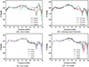 |
Figure 16. Effect of radiating head parameters on transmitting voltage response. (a) Outer radius. (b) Radiating head thickness. (c) Slot width. (d) Slot depth. |
The simulation results are shown in Figure 17, where the main thickness e, front-end thickness f, bolt insertion depth g, and platform length h are sequentially varied. In Figure 17a, the response curve fluctuates minimally as the main thickness increases. The overall trend is a decrease followed by an increase, with the transmitting voltage response rising after 34–40 kHz and again after 45 kHz. In Figure 17b, as the front-end thickness increases, the transmitting voltage response generally becomes smoother, but at 10.5 mm, the fluctuation increases. Therefore, this dimension should not be excessively large. Figure 17c indicates that as the bolt insertion depth increases, the transmitting voltage response continues to decrease in the frequency range above 34 kHz, with minimal overall impact on the curve. Finally, Figure 17d shows that increasing the platform length causes an upward shift in the curve between the second and third resonant frequencies.
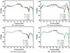 |
Figure 17. Effect of front cover parameters on transmitting voltage response. (a) Main thickness. (b) Front-end thickness. (c) Bolt insertion depth. (d) Platform length. |
To further quantify the optimization effects, the influence of dimensional parameters on the response peak values at each resonant frequency is summarized in Table 3, where arrows indicate the increase or decrease of the resonance peaks.
Effect of dimensional variations on response peaks at resonant frequencies.
In summary, with other structural materials held constant, the dimensions of the Tonpilz transducer mass blocks, front cover, and radiating head have been optimized. The thicknesses of the front, middle, and rear mass blocks are all 8 mm, while the outer radius a, radiating head thickness b, slot width c, and slot depth d of the radiating head are 43 mm, 12 mm, 8 mm, and 7.5 mm, respectively. The main thickness e, front-end thickness f, bolt insertion depth g, and platform length h of the front cover are 31 mm, 8.5 mm, 12 mm, and 11.5 mm, respectively. Under these optimized conditions, the transducer achieves a smooth transmitting voltage response across the desired frequency band. As shown in Figure 18, when the transducer operates in a partial excitation mode, its operating frequency range is from 17 kHz to 41 kHz, with a −3 dB bandwidth of 24 kHz. The maximum transmitting voltage response within this bandwidth is 143.7 dB re 1 μPa/V @ 1 m, occurring at a frequency of 36 kHz.
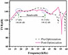 |
Figure 18. Transmitting voltage response after dimensional optimization. |
Figure 19 illustrates the radiation directivity of the optimized transducer at three resonant frequencies within the operating bandwidth. The simulation settings are consistent with those in Figure 12. At 17.4 kHz, 31.8 kHz, and 36.0 kHz, the far-field −3 dB beamwidths are 57.32°, 40.89°, and 70.11°, respectively. Compared to the pre-optimization case, the beamwidths at the first and third resonant frequencies decrease, while the beamwidth at the second resonant frequency increases. Modal analysis in Section 4.3 and the vibration characteristics of the transducer show that the first resonant frequency is dominated by longitudinal vibration of the radiating head and piezoelectric ceramic stack, producing acoustic radiation characteristics similar to ideal piston-like radiation. At the second resonant frequency of 31.6 kHz, the −3 dB beamwidth increases, indicating a more dispersed energy distribution. At the third resonant frequency of 36 kHz, the −3 dB beamwidth reaches its maximum, exhibiting a broad main lobe and multiple side lobes, reflecting the complexity of vibration modes at this frequency.
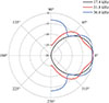 |
Figure 19. Radiation pattern at different resonant frequencies within the bandwidth. |
Table 4 presents a detailed comparison of the simulation performance of the transducer in this study with other published results. The comparison includes key parameters such as cavity shape, −3 dB beamwidth, maximum transmitting voltage response (Max TVR) within the bandwidth, center frequency, −3 dB operating bandwidth (−3 dB Operating BW), and band-width improvement (BW Improvement). The −3 dB beamwidth compared in this table refers to the angular span of the main radiation lobe, measured at the points where the response is 3 dB below the peak at the Max TVR frequency. Bandwidth improvement represents the percentage increase in transducer bandwidth in this study relative to the simulated bandwidth of other transducers, expressed as follows
Performance comparison of transducers.
 (6)
(6)
where BWprop is the bandwidth of the proposed transducer and BWlit is the bandwidth of the transducer from the literature.
The comparison results indicate that the Tonpilz transducer in this study is competitive in several key metrics compared to other transducers in the table. Within the bandwidth range, the maximum transmitting voltage response is 143.7 dB re 1 μPa/V @ 1 m, the −3 dB operating bandwidth extends to 24 kHz, and good sound wave directivity is maintained while achieving a wide bandwidth.
6 Conclusion
The finite element method was applied to optimize and analyze multi-driven Tonpilz transducer performance, with a focus on excitation methods and structural design. A multi-driven underwater Tonpilz transducer with a radiating head containing concentric-ring cavities was proposed, in which the cavities reduce effective mass and enhance bandwidth. Analysis of three excitation methods of the piezoelectric ceramic stack, in-phase, anti-phase, and partial excitation, revealed that partial excitation effectively excites the first three resonant modes while maintaining favorable admittance characteristics, achieving optimal transducer performance. Furthermore, impedance characteristics in water were investigated, and modal and directivity analyses clarified the vibration behavior of each mode and the corresponding beamwidth. Finally, to reduce fluctuations in transmitting voltage response over the 18–40 kHz range, the effects of mass block, radiating head, and front cover dimensions were evaluated. After optimization, the transducer operates over 17 kHz–41 kHz, with a −3 dB bandwidth of 24 kHz and a maximum transmitting voltage response of 143.7 dB re 1 μPa/V @ 1 m, demonstrating significantly enhanced performance.
Funding
This work was supported by the National Key Research and Development Program of China (Grant No.2024YFB4710803) and the National Natural Science Foundation of China (Grant No.12404528).
Conflicts of interest
The authors declare no conflict of interest.
Data availability statement
Data are available on request from the authors.
References
- R.A.G. Fleming, D.F. Jones, C.G. Reithmeier: Broadband cluster transducer for underwater acoustics applications. The Journal of the Acoustical Society of America 126, 5 (2009) 2285–2293. [Google Scholar]
- S.E. Freeman, L.E. Emokpae, G.F. Edelmann: High-frequency, highly directional short-range underwater acoustic communications, in: OCEANS 2015 MTS/IEEE Washington. IEEE, 2015, 1–4. [Google Scholar]
- Z. Abdullah, S. Naz, M.A.Z. Raja, A. Zameer: Design of wideband tonpilz transducers for underwater SONAR applications with finite element model. Applied Acoustics 183 (2021) 108293. [Google Scholar]
- J.Y. Pyun, Y.H. Kim, K.K. Park: Design of piezoelectric acoustic transducers for underwater applications. Sensors 23, 4 (2023) 1821. [Google Scholar]
- T. Theocharidis, E. Kavallieratou: Underwater communication technologies: a review. Telecommunication Systems 88 (2025) 54–67. [Google Scholar]
- H.C. Song, W.S. Hodgkiss: Efficient use of bandwidth for underwater acoustic communication. The Journal of the Acoustical Society of America 134 (2013) 905–908. [Google Scholar]
- Z. Li, M. Chitre, M. Stojanovic: Underwater acoustic communications. Nature Reviews Electrical Engineering 2, 2 (2025) 83–95. [Google Scholar]
- Y. Roh, Y. Lim: Tonpilz-type vector sensor for the estimation of underwater sound wave direction. The Journal of the Acoustical Society of America 144, 5 (2018) 2801–2810. [Google Scholar]
- D. Teng: Z-structured piezoelectric transducers: a new approach for low-frequency small-size underwater projectors. IEEE Sensors Journal 23, 4 (2023) 3514–3520. [Google Scholar]
- R. Villalobos, H. López, N. Vázquez, R.V. Carrillo-Serrano, A. Espinosa-Calderón: Cavitation detection in a Tonpilz-type transducer for active SONAR transmission system. Journal of Marine Science and Engineering 11, 7 (2023) 1279. [Google Scholar]
- M. Hadeed, H.S. Bhatti, M.S. Afzal, V. Epin, M. Abdullah: Design and development of a high-power wideband multimode Tonpilz transducer for underwater applications. Journal of Mechanical Engineering and Sciences 18, 3 (2024) 10161–10170. [Google Scholar]
- J. Kim, J. Kim, J. Kang: Advances in Langevin piezoelectric transducer designs for broadband ultrasonic transmitter applications. Actuators 14, 7 (2025) 150. [Google Scholar]
- Q. Liu, J. Li, K. Yang, M.S. Wang: Research on a multimode wideband Tonpilz transducer, in: 2022 16th Symposium on Piezoelectricity, Acoustic Waves, and Device Applications (SPAWDA). IEEE, 2022, pp. 248–252. [Google Scholar]
- D.W. Hawkins, P.T. Gough: Multiresonance design of a Tonpilz transducer using the finite element method. IEEE Transactions on Ultrasonics, Ferroelectrics, and Frequency Control 43, 5 (1996) 782–790. [Google Scholar]
- Q. Yao, L. Bjorno: Broadband Tonpilz underwater acoustic transducers based on multimode optimization. IEEE Transactions on Ultrasonics, Ferroelectrics, and Frequency Control 44, 5 (1997) 1060–1066. [Google Scholar]
- P. Kurt, M. Şansal, I. Tatar, C. Duran, S. Orhan: Vibro-acoustic design, manufacturing and characterization of a tonpilz-type transducer. Applied Acoustics 150 (2019) 27–35. [Google Scholar]
- S.C. Thompson: Broadband multi-resonant longitudinal vibrator transducer. U.S. Patent 4633119, 1986. [Google Scholar]
- C.H. Sherman, J.L. Butler: Transducers and Arrays for Underwater Sound. Springer, New York, 2007. [Google Scholar]
- J.L. Butler, S.C. Butler, A.E. Clark: Unidirectional magnetostrictive/piezoelectric hybrid transducer. The Journal of the Acoustical Society of America 88, 1 (1990) 7–11. [Google Scholar]
- A.L. Butler, J.L. Butler: Broadband acoustic transducer with multiple resonant modes. U.S. Patent 6950373, 2005. [Google Scholar]
- K. Zhang, W. Li, J. Wang, H. Chen: Research on the broadband dual-excited underwater acoustic transducer. Advanced Engineering Forum 2–3 (2011) 144–147. [Google Scholar]
- S. Pyo, M.S. Afzal, Y. Lim, S. Lee, Y. Roh: Design of a wideband tonpilz transducer comprising non-uniform piezoceramic stacks with equivalent circuits. Sensors 21, 8 (2021) 2680. [Google Scholar]
- B. Ji, Y. Lan, G. Qiao, S. Shao: Experimental investigation of a Tonpilz transducer operating in the frequency band of 20–80 kHz (L). The Journal of the Acoustical Society of America 155, 6 (2024) 3600–3603. [Google Scholar]
- B. Ji, L. Hong, Y. Lan: Influences of length and position of drive-stacks on the transmitting-voltage-response of the broadband Tonpilz transducer. The Journal of the Acoustical Society of America 150, 6 (2021) 4140–4150. [Google Scholar]
- Z.Q. Li, X.P. Mo, Y.M. Li, Y.Z. Pan: Analysis of double-excited piezoelectric Tonpilz transducer, in: 2013 Symposium on Piezoelectricity, Acoustic Waves, and Device Applications. IEEE, 2013, 1–4. [Google Scholar]
- X. He, X. Zhu, Z. Wu, X. Kang, Y. Wang: A wideband tonpilz transducer with a transverse through-hole in the radiating head. The Journal of the Acoustical Society of America 150, 4 (2021) 2655–2663. [Google Scholar]
- X. He, J. Hu: Study on the broadband tonpilz transducer with a single hole. Ultrasonics 49, 4, 5 (2009) 419–423. [Google Scholar]
- H. Kim, Y. Roh: Design and fabrication of a wideband Tonpilz transducer with a void head mass. Sensors and Actuators A: Physical 239 (2016) 137–143. [Google Scholar]
- S. Chhith, Y. Roh: Wideband Tonpilz transducer with a cavity inside a head mass. Japanese Journal of Applied Physics 49, 7S (2010) 07HG08. [Google Scholar]
- H.-W. Ji, A.Q. Qi, F. Yang, X. Wu, B. Lv, J. Ni: Design of acoustic impedance gradient matching layers. Applied Acoustics 211 (2023) 109549. [Google Scholar]
- J. Bian, Y. Wang, Z. Liu, M. Shen, H. Zhao, Y. Sun, J. Zhu: Ultra-wideband underwater acoustic transducer with a gradient impedance matching layer. Applied Acoustics 175 (2021) 107789. [Google Scholar]
- V.T. Rathod: A review of acoustic impedance matching techniques for piezoelectric sensors and transducers. Sensors 20 (2020) 4051. [CrossRef] [PubMed] [Google Scholar]
- E.S. Røed, M. Bring, F. Tichy, A. Henriksen, E.M. Åsjord, L. Hoff: Optimization of matching layers to extend the usable frequency band for underwater single-crystal piezocomposite transducers. IEEE Transactions on Ultrasonics, Ferroelectrics, and Frequency Control 69 (2021) 803–811. [Google Scholar]
- D. Stansfield, A. Elliott: Underwater Electroacoustic Transducers. Peninsula Publishing, 2017. [Google Scholar]
- D. Rajapan: Performance of a low-frequency, multi-resonant broadband Tonpilz transducer. The Journal of the Acoustical Society of America 111, 4 (2002) 1692–1694. [Google Scholar]
- J.L. Butler, J.R. Cipolla, W.D. Brown: Radiating head flexure and its effect on transducer performance. The Journal of the Acoustical Society of America 70, 2 (1981) 500–503. [Google Scholar]
- R. Jiang, L. Mei, Q.M. Zhang: COMSOL multiphysics modeling of architected acoustic transducers in oil drilling. Mrs Advances 1, (2016) 1755–1760. [Google Scholar]
- Y. Gao, M.H. Zhu: Application of the Reflectionless Discrete Perfectly Matched Layer for Acoustic Wave Simulation. Frontiers in Earth Science 10 (2022) 883160. [Google Scholar]
- F. Ihlenburg, Ed.: Finite Element Analysis of Acoustic Scattering. Springer, New York, 1998. [Google Scholar]
- Z.Q. Li, X.P. Mo, Y.Z. Pan, Y.P. Liu: Design and analysis of a longitudinal piezoelectric vibration exciter, in: 2012 Symposium on Piezoelectricity, Acoustic Waves, and Device Applications. IEEE (2012) 155–158. [Google Scholar]
- C. Wang, Y. Lan, W. Cao: Tonpilz transducer head mass selection based on excitation signal type. Applied Acoustics 176 (2021) 107852. [Google Scholar]
- J.L. Butler, A.L. Butler: Ultra wideband multiple resonant transducer, in: Oceans 2003. Celebrating the Past... Teaming Toward the Future. Vol. 5. IEEE (2003) 2381–2387. [Google Scholar]
- H.S. Ju, Y.H. Kim: Near-field characteristics of the parametric loudspeaker using ultrasonic transducers. Applied Acoustics 71, 9 (2010) 793–800. [CrossRef] [Google Scholar]
- N. Sheida, H.M. Sedighi, A. Valipour: Identification and estimation of the bandwidth of different acoustic arrays composed of Tonpilz transducers in engineering sonar systems. Journal of Engineering Management and Systems Engineering 4, 2 (2025) 133–160. [Google Scholar]
Cite this article as: Xue K. Zhu Y. Wang S. Zhang C. Bao Z. & Li N. 2025. Finite element optimization and performance analysis of a multi-driven Tonpilz transducer. Acta Acustica, 9, 76. https://doi.org/10.1051/aacus/2025060.
All Tables
All Figures
|
Figure 1. Traditional Tonpilz underwater acoustic transducer structure. |
| In the text | |
|
Figure 2. Schematic diagram of the head mass with cavity. |
| In the text | |
|
Figure 3. Schematic diagram of the connection between the radiating head and the front cover in practical applications. |
| In the text | |
|
Figure 4. Schematic diagram of the multi-driven Tonpilz transducer with a radiating head containing concentric-ring cavities. |
| In the text | |
|
Figure 5. Schematic diagram of polarization directions and electrical connections of piezoelectric ceramic rings. |
| In the text | |
|
Figure 6. Transducer finite element mesh. |
| In the text | |
|
Figure 7. Different excitation methods of the piezoelectric ceramic stacks. (a) In-phase excitation. (b) Anti-phase excitation. (c) Partial excitation. |
| In the text | |
|
Figure 8. Transmitting voltage response under different excitation methods. |
| In the text | |
|
Figure 9. Admittance and resonant modes of the Tonpilz transducer in air under different excitation methods. (a) Admittance of the transducer under in-phase excitation. (b) Admittance of the transducer under anti-phase excitation. (c) Admittance of the transducer under partial excitation. (d) Amplified admittance curve under 34.6 kHz anti-phase excitation. |
| In the text | |
|
Figure 10. Transducer conductance-susceptance result. |
| In the text | |
|
Figure 11. Vibration modes of the transducer under water loading. (a) First resonance – 19.3 kHz. (b) Second resonance – 34.9 kHz. (c) Third resonance – 40.2 kHz. (d) Fourth resonance – 51.5 kHz. |
| In the text | |
|
Figure 12. Radiation pattern of the transducer at different resonant frequencies. |
| In the text | |
|
Figure 13. Transmitting voltage response before optimization. |
| In the text | |
|
Figure 14. Effect of mass block thickness on transmitting voltage response. (a) Front mass block. (b) Middle mass block. (c) Rear mass block. |
| In the text | |
|
Figure 15. 2D symmetric geometry and 3D modeling of the front cover and radiating head. |
| In the text | |
|
Figure 16. Effect of radiating head parameters on transmitting voltage response. (a) Outer radius. (b) Radiating head thickness. (c) Slot width. (d) Slot depth. |
| In the text | |
|
Figure 17. Effect of front cover parameters on transmitting voltage response. (a) Main thickness. (b) Front-end thickness. (c) Bolt insertion depth. (d) Platform length. |
| In the text | |
|
Figure 18. Transmitting voltage response after dimensional optimization. |
| In the text | |
|
Figure 19. Radiation pattern at different resonant frequencies within the bandwidth. |
| In the text | |
Current usage metrics show cumulative count of Article Views (full-text article views including HTML views, PDF and ePub downloads, according to the available data) and Abstracts Views on Vision4Press platform.
Data correspond to usage on the plateform after 2015. The current usage metrics is available 48-96 hours after online publication and is updated daily on week days.
Initial download of the metrics may take a while.