| Issue |
Acta Acust.
Volume 9, 2025
|
|
|---|---|---|
| Article Number | 67 | |
| Number of page(s) | 15 | |
| Section | Ultrasonics | |
| DOI | https://doi.org/10.1051/aacus/2025052 | |
| Published online | 31 October 2025 | |
Scientific Article
Determination of acoustic field parameters for high-frequency focusing ultrasonic transducers up to 100 MHz
1
Division of Mechanics and Acoustics, National Institute of Metrology, Beijing, 100029, PR China
2
Jiangsu Institute of Medical Device Testing, Nanjing, 210019, PR China
* Corresponding authors: This email address is being protected from spambots. You need JavaScript enabled to view it.
; This email address is being protected from spambots. You need JavaScript enabled to view it.
Received:
13
August
2025
Accepted:
1
October
2025
Abstract
High-frequency focused ultrasonic technology offers distinct advantages in microstructural inspection and high-resolution imaging owing to its short wavelength and superior acoustic field-focusing capability. Accurate determination of focused acoustic field characteristics is essential for reliable defect evaluation and image quality. This study proposes a precise method for calibrating the effective radius of high-frequency focusing ultrasonic transducer and −6 dB beamwidth of its acoustic field – two key parameters that directly affect the spatial resolution and focusing accuracy. A theoretical acoustic field model was established based on the Rayleigh integral, and the computational efficiency was enhanced using the Fresnel approximation. A hydrophone-based experiment was designed: the iterative method was employed to invert the geometric focal length and effective radius by analyzing the extrema (maximum and minimum values) of the on-axis acoustic pressure distribution, while the −6 dB beamwidth was determined by incorporating a spatial averaging correction into the analysis of the focal plane pressure profile. The experimental results demonstrate that the determined beamwidths agree with the measured values to within 3% across a frequency range of up to 100 MHz, thereby confirming the accuracy, robustness and practical applicability of the proposed calibration approach.
Key words: Beamwidth / Effective radius / Focal length / Focusing transducer
© The Author(s), Published by EDP Sciences, 2025
 This is an Open Access article distributed under the terms of the Creative Commons Attribution License (https://creativecommons.org/licenses/by/4.0), which permits unrestricted use, distribution, and reproduction in any medium, provided the original work is properly cited.
1 Introduction
With the continuous advancement of modern industrial manufacturing and intelligent inspection technologies, increasingly stringent requirements have been imposed on real-time and high-precision evaluation of material properties and structural integrity, particularly in high-tech fields such as aerospace [1], microelectronic packaging, and biomedical devices. The demands for spatial resolution, penetration depth, and adaptability to multi-physical coupling environments in inspection technologies have exhibited exponential growth trends [2–4]. Traditional nondestructive testing (NDT) methods, such as radiographic testing [5] and eddy current testing [6], present notable limitations in detecting micro-defects, identifying inner-layer defects in complex structures, and multi-physical field coupling scenarios. These limitations may include insufficient resolution, limited penetration capability, and poor sensitivity to variations in the material properties.
In contrast, ultrasonic testing has emerged as a mainstream NDT technique in modern industry, because of its non-invasiveness [7], excellent time-domain resolution, high sensitivity [8] to deeply embedded defects, and ease of integration into real-time monitoring systems. Notably, high-frequency focusing ultrasound exhibits distinct advantages in applications such as hydrophone calibration [9], microstructural evaluation, high-resolution imaging (e.g., ultrasonic microscopy), and inspection of integrated circuit packages, owing to its short wavelength and superior acoustic field focusing capability. As the core component of an ultrasonic inspection system, the transducer directly determines the detection sensitivity and the spatial resolution of the system. The quantitative characterization of its acoustic field parameters not only influences the reliability of defect evaluation, but is also critical for verifying compliance with international standards such as ASTM [10] and ISO [11].
In ultrasonic NDT, accurate modeling of acoustic field and precise calibration of key parameters of the transducer form the foundation for system design optimization, imaging algorithm development, and quantitative defect assessment. Among these, the beamwidth and effective radius are key indicators for evaluating the performance of focusing transducers. These parameters directly affect the spatial resolution and focusing precision. Even slight deviations can significantly influence defect characterization, potentially resulting in false positives or missed detections. Knowledge of these parameters can also be applied to perform spatial averaging corrections in hydrophone calibration [12–15]. Therefore, the development of reliable measurement and calibration techniques is vital.
The beamwidth is typically defined as the full width at the −6 dB level (i.e., the half-maximum) of the acoustic pressure amplitude or intensity distribution at the focal plane, and serves as a measure of the transducer’s lateral resolution [16]. However, high-frequency focusing transducers exhibit considerably shorter wavelengths than their low-frequency counterparts. Conventional measurement techniques, such as hydrophone-based acoustic pressure acquisition, are increasingly affected by the spatial averaging effect [17, 18], particularly when the hydrophone’s aperture is comparable to or larger than the beamwidth. Under such conditions, the hydrophone can no longer be approximated as an ideal-point receiver, leading to significant errors in the field characterization. The effective radius, representing the actual emitting area contributing to the acoustic field distribution [19], is a critical input parameter for theoretical modeling methods, such as Rayleigh integral and Fresnel approximation. As the frequency increases, the signal-to-noise ratio (SNR) decreases, particularly in the pre-focal range, where the fluctuating characteristics of the acoustic field are difficult to measure accurately. This limitation reduces the applicability of certain calibration algorithms, such as the two-axial-node method [20], and significantly constrains available calibration methods under high-frequency conditions. Moreover, high-frequency acoustic field measurements suffer from additional challenges, including hydrophone positioning errors [21, 22] and bandwidth limitations of the transducer, further complicating the reliable determination of the acoustic field parameters.
To address these challenges, this study proposes an iterative inversion method to reconstruct the geometric focal length of the transducer, thereby enabling the calibration of the effective radius and determination of the −6 dB beamwidth. By integrating theoretical modeling with experimental validation, the key acoustic field characteristics of high-frequency focusing ultrasonic transducers are determined precisely. First, the focused acoustic field was theoretically modeled based on the Rayleigh integral, with computational simplification achieved through a series expansion and application of the Fresnel approximation. This resulted in an acoustic pressure distribution model tailored to high-frequency focused transducers. Subsequently, a hydrophone-based calibration experiment was designed and implemented. To resolve notable discrepancies encountered when employing the acoustic focal length in the effective radius calibration method, an algorithm was developed to iteratively invert the geometric focal length by analyzing the maxima and minima of the on-axis acoustic pressure distribution. This enabled the accurate calibration of the effective radius. Furthermore, the −6 dB beamwidth was determined by incorporating the spatial averaging effect into the analysis of the pressure distribution within the focal plane. This approach allows for a comprehensive and quantitative evaluation of acoustic focusing performance. The experimental results show close agreement up to 100 MHz, providing essential technical support for acoustic field modeling, transducer parameter optimization, and enhanced accuracy of ultrasonic imaging algorithms.
2 Theory
This study analyzes the radiated acoustic field characteristics of focusing ultrasonic transducers under the framework of the linear acoustic theory, based on the following fundamental assumptions:
-
(a)
The propagation medium is treated as an ideal, inviscid fluid;
-
(b)
The medium is initially homogeneous and stationary;
-
(c)
The acoustic waves satisfy the small-amplitude vibration condition.
The focusing ultrasonic transducer is modeled as a circular piston source mounted on an infinite rigid baffle, characterized by radius a, geometric focal length F, and spherical cap height h. The transducer surface is assumed to oscillate uniformly with a constant velocity amplitude V. To prevent the propagation of Lamb waves in the transducer emitting surface, the transducer element is fabricated using a piezoelectric composite material [23].
As illustrated in Figure 1, a three-dimensional Cartesian coordinate system is defined with origin O located at the center of the transducer surface. The acoustic axis aligns with the positive z-axis, and the geometric focus is denoted as point R. Let q represent a radiation point on the transducer surface. The angle between the line connecting q, the focal point R and the acoustic axis is defined as θ0. Within the plane containing the radiation point q and parallel to the XY plane, the angle between the line connecting the intersection of this plane with the acoustic axis and point q and the x-axis is defined as φ. The semi-aperture angle of the focusing transducer is given by β = arcsine(a/F). At the receiving end, a hydrophone with radius b is positioned in a plane perpendicular to the acoustic axis at a distance r from the transducer. The lateral offset between the hydrophone center O′ and the acoustic axis is denoted by x. The receiving point Q is defined on the hydrophone surface, with the radial distance from the hydrophone center expressed as η. The angle between this line and the x-axis is denoted by ϕ. The distance between the radiation point q and the receiving point Q is represented by r′.
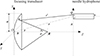 |
Figure 1 Measurement of the acoustic field of a focusing transducer using a needle hydrophone. |
The acoustic pressure at the receiving point Q is expressed as follows [24]:
 (1)
(1)
In the above integral expression of acoustic pressure, the influence of secondary diffraction on the focal plane is neglected.
The average acoustic pressure measured by the hydrophone is:
 (2)
(2)
where A b denotes the effective area of the hydrophone.
The distance between radiation point q and receiving point Q is
![Mathematical equation: $$ \begin{aligned} r^{\prime } = \left\{ \begin{aligned} {r^2}&+ {\eta ^2} + 2\eta r\sin \theta \cos \phi \\&+ 2{F^2}\Bigg [\left(1 - \cos \theta _0\right)\left(1 - \frac{{r\cos \theta }}{F}\right) \\ &- \frac{\eta }{F}\sin \theta _0\cos (\varphi + \phi ) \\ &- \frac{{r\sin \theta }}{F}\sin \theta _0\cos \varphi \Bigg ]\end{aligned}\right\} ^{\frac{1}{2}}. \end{aligned} $$](/articles/aacus/full_html/2025/01/aacus250118/aacus250118-eq3.gif) (3)
(3)
2.1 On-axis acoustic pressure distribution
Along the acoustic axis, r = z, θ = 0. Equation (3) can be simplified to
![Mathematical equation: $$ \begin{aligned} r^{\prime } = \left\{ \begin{aligned} {z^2}&+ {\eta ^2} + 2{F^2}\Bigg [\left(1 - \cos \theta _0\right)\left(1 - \frac{z}{F}\right) \\ &- \frac{\eta }{F}\sin \theta _0\cos (\varphi + \phi )\Bigg ]\end{aligned}\right\} ^{\frac{1}{2}}. \end{aligned} $$](/articles/aacus/full_html/2025/01/aacus250118/aacus250118-eq4.gif) (4)
(4)
Substituting equation (4) into equation (2) yields an exact expression for the on-axis acoustic pressure of the focusing transducer as measured by the hydrophone. To simplify the radiation integral, Fresnel approximation is applied. Specifically, the distance r′ in the denominator is approximated by z and the exponential term is expanded using a Taylor series, retaining only the first two terms. This leads to the following simplified form:
![Mathematical equation: $$ \begin{aligned} r^{\prime } \approx &z + \frac{\eta }{{2z}} \\&+ \frac{{{F^2}}}{z}\left[(1 - \cos \theta _0)\left(1 - \frac{z}{F}\right) - \frac{\eta }{F}\sin \theta _0\cos (\varphi + \phi )\right].\nonumber \end{aligned} $$](/articles/aacus/full_html/2025/01/aacus250118/aacus250118-eq5.gif) (5)
(5)
In addition, by exploiting the periodicity of the cosine function, the integration over angle φ is eliminated. Consequently, under the Fresnel approximation, the average acoustic pressure measured by the hydrophone is simplified as:
 (6)
(6)
Figure 2 presents the numerically computed on-axis acoustic pressure distributions of the focusing ultrasonic transducers when measured with needle hydrophones of varying diameters. Simulations were conducted for the following transducers: (a) an Olympus 30 MHz focusing transducer (V375) with a nominal radius of 0.125 inch and a focal length of 0.75 inch; (b) a NIM 75 MHz focusing transducer (NO.4550377) with a nominal radius of 1.5 mm and a focal length of 12 mm. The normalized distance z/F is used as the abscissa to ensure that geometric focal length is always represented at 1. As shown in Figure 2, increasing the hydrophone diameter leads to a pronounced reduction of the measured acoustic pressure amplitude. When the hydrophone diameter exceeded a critical threshold, the on-axis pressure distribution deviated substantially from the ideal reference curve, exhibiting significant distortion owing to the spatial averaging effect.
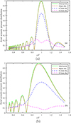 |
Figure 2 On-axis acoustic pressure distribution of focusing transducers measured by different hydrophones. (a) Focusing transducer at 30 MHz (nominal radius 0.125 inch). (b) Focusing transducer at 75 MHz (nominal radius 3 mm). |
2.1.1 Calibration of effective radius
In this study, a theoretical acoustic field model is constructed based on surface integral formulations over the radiating aperture of a focusing ultrasonic transducer, enabling the simulation of its spatial acoustic pressure distribution. For a spherically focusing transducer, the acoustic field characteristics are predominantly governed by the effective emission area that actively contributes to acoustic radiation. Therefore, the accurate calibration of the effective radius a eff is crucial, as it serves as a key input parameter in Rayleigh integral formulations or their approximations.
Notably, a eff often deviates from the geometric or nominal radius provided by the manufacturer. This deviation arises from factors such as non-ideal vibration boundaries, inhomogeneous acoustic impedance across the piezoelectric surface, and frequency-dependent response characteristics. Because the direct determination of a eff from manufacturing parameters is typically infeasible, this study proposes a parameter inversion method that integrates acoustic field measurements with theoretical fitting. Specifically, the transducer is driven by burst excitation, and the on-axis acoustic pressure distribution is measured in water. The effective radius a eff is then calibrated and extracted by leveraging the functional relationship between the on-axis acoustic pressure in the theoretical model and the effective radius of the transducer. Combined measurement and modeling approaches were also used in high intensity focused ultrasound applications to determine the effective radius of transducers, which then in turn was used as input parameter for non-linear field modeling [25, 26].
Further examination of the on-axis acoustic pressure distributions presented in Figure 2 reveals pronounced periodic oscillations in the pre-focal range adjacent to the transducer. These oscillations are characterized by alternating local maxima and minima resulting from the combined effects of acoustic interference and diffraction, which dominate the spatial behavior of the focused field in this region. Notably, when the physical dimensions of the hydrophone’s sensing surface are of the order of the acoustic wavelength, the spatial averaging effect significantly compromises the measurement accuracy, causing the measured acoustic pressure distribution to deviate from theoretical expectations.
To analyze the on-axis acoustic field characteristics of the focusing transducer more accurately, an ideal-point receiver model is introduced. This model assumes that the spatial dimension of the receiver approaches infinitesimal, enabling it to truly reflect the acoustic pressure value at each spatial point without being affected by the probe size or response characteristics. Under this assumption, the on-axis acoustic pressure distribution of a spherical focusing transducer has a well-defined analytical expression. The corresponding expression for the pressure field received by the ideal point receiver is given as [24]:
 (7)
(7)
where B(z) is the distance from the point receiver on the acoustic axis to the spherical edge of the focusing transducer, as shown in Figure 3. According to the geometric structure of the focusing transducer, the following can be obtained that:
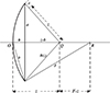 |
Figure 3 Schematic diagram of geometric structure of focusing transducer. |
 (8)
(8)
According to equation (8), the positions of the on-axis acoustic pressure minima are at
 (9)
(9)
Solving for z, a series of positions of the minimum points denoted as z n is obtained as follows:
 (10)
(10)
where “+2n λ” in the denominator corresponds to the minimum points located before the transducer’s geometric focus F, while the “−2n λ” corresponds to those after the geometric focus F. As n increases, these positions become progressively farther from the geometric focus F.
Owing to the severe attenuation of high-frequency signals during propagation in the medium, the signal-to-noise ratio is significantly reduced. Experimental observations revealed that distinguishable fluctuations in the acoustic field are difficult to observe in the pre-focal range adjacent to the transducer. Typically, only the first pressure minimum near the focal length and subsequent secondary maximum can be clearly identified. Accordingly, by considering the minimum pressure closest to the geometric focus F on the transducer side (n = 1), its axial position can be expressed as:
 (11)
(11)
The parameter h can be approximated as:
 (12)
(12)
where the geometric focal length F is much greater than the radius a (F ≫ a). For ultrasonic transducers employed in non-destructive testing, particularly high-frequency focusing transducers, the wave number k is typically large. Under this condition, an approximate expression for the effective radius can be derived from equation (11) in a simplified form: this approximation is adopted as the effective radius a eff and is expressed as follows:
 (13)
(13)
It can be inferred from equation (13), which measures only the on-axis pressure minimum position z min, is insufficient for determining the effective radius a eff of a spherically focusing transducer. This is because a eff also depends explicitly on the transducer’s geometric focal length F (i.e., radius of curvature of the spherical surface). Any deviation in the value of the focal length F directly affects the effective radius inverted from the theoretical model, thereby compromising the overall precision and repeatability of the acoustic field calibration.
An observation of the on-axis pressure distribution curves shown in Figure 2 reveals that the location of the actual acoustic focus, defined as the point at which the on-axis acoustic pressure reaches its maximum, does not exactly coincide with the geometric focus of the transducer. The analysis of the on-axis acoustic pressure expression shown in equation (7) reveals that the acoustic pressure magnitude is governed by the combined effect of an amplitude modulation term and phase modulation term. For convenience in subsequent calculations, according to equation (8), z can be expressed as [27]:
 (14)
(14)
By substituting equation (14) into equation (7), the following expression is obtained:
 (15)
(15)
where  . According to the Taylor series expansion of the sine function:
 (16)
(16)
Equation (15) can be expanded as:
![Mathematical equation: $$ \begin{aligned} \left| {P_a} \right| = 2\rho cV\left[ {kh + Nk\delta (z) - \left(\frac{{kh}}{{3!}} + \frac{{2N}}{{kF}}\right){{\left(\frac{{k\delta (z)}}{2}\right)}^2} - \cdots } \right]. \end{aligned} $$](/articles/aacus/full_html/2025/01/aacus250118/aacus250118-eq18.gif) (17)
(17)
Although the amplitude term in the on-axis acoustic pressure distribution is frequency independent, it can be expressed in terms of k h, k δ and k F, as shown in equation (17). Therefore, the on-axis acoustic pressure distribution can be regarded as a function of k δ, and the positions of its maximum points coincide with the roots of P a′(k δ)=0:
![Mathematical equation: $$ \begin{aligned} P_a^{\prime }(k\delta ) = 2\rho cV\left[ {N - \left(\frac{{kh}}{{3!}} + \frac{{2N}}{{kF}}\right)\frac{{k\delta (z)}}{2} - \cdot \cdot \cdot } \right]. \end{aligned} $$](/articles/aacus/full_html/2025/01/aacus250118/aacus250118-eq19.gif) (18)
(18)
At the geometric focal length F of the transducer, z = F = B(z), δ(z)=0, P a ′(k δ)=2ρ c V N ≠ 0 is clearly not the location of the maximum acoustic pressure. The k δ max corresponding to the acoustic pressure maximum point is the smallest positive root of the equation P a′(k δ)=0, which can be approximated as
 (19)
(19)
Substituting into equation (14), the corresponding z max is obtained as:
 (20)
(20)
The maximum point of the on-axis acoustic pressure is typically located slightly anterior to the geometric focal length F of the transducer, and its location is primarily governed by the dimensionless parameter k h. Consequently, the actual acoustic focus is influenced not only by the excitation frequency f, but also by the structural parameters of the transducer. As k h increases, the axial maximum pressure position z max gradually converges toward the geometric focus F of the spherical focusing transducer. For high-frequency focusing transducers, although the wave number k is inherently large, the geometric parameter h is often small, owing to the structural limitations of compact transducer designs. As a result, the product k h cannot always be considered sufficiently large, and the correction term associated with the actual focal position becomes non-negligible. This term often introduces positional deviations of the order of several percent. Given that the focal length and −6 dB beamwidth of high-frequency transducers typically fall within the millimeter or even sub-millimeter range, such small deviations may lead to substantial errors in the inversion of the effective radius. Therefore, these corrections must be carefully considered for precise acoustic field determination.
In experimental measurements, the position of the on-axis acoustic pressure maximum z max can typically be obtained with relatively high accuracy, whereas the geometric focal length F of the transducer cannot be directly measured. The geometric focal length is usually specified and labeled by the transducer manufacturer during production, and may be indicated in the factory inspection report or device housing. If an accurate geometric focal length F of the focusing transducer is available, the effective radius can be calibrated by simply measuring the position of the minimum point z min. However, there is no unified standard for labeling specifications across manufacturers – some nominal “focal lengths” refer to the actual maximum acoustic pressure position rather than the geometric focus. Moreover, the actual transducer structure often deviates from the ideal: installation errors in wafer positioning, inconsistencies in backing layer thickness, and long-term aging of piezoelectric materials can all introduce deviations in geometric parameters, such as the radius of curvature, resulting in discrepancies between the labeled and actual values.
In most experimental scenarios, researchers can readily obtain the positions of the on-axis acoustic pressure maximum z max and first minimum z min. These two characteristic points can be expressed as functions of a eff and F using equations (13) and (20), respectively. In theory, combining the information from these two measurements allows for analytical inversion of a eff. However, this leads to a transcendental equation involving F that precludes the derivation of a closed-form solution. To address this issue, this study proposes an iterative optimization algorithm as an approximate solution. Based on equation (13), the initial geometric focal length is set as the measured acoustic pressure maximum zmax, and the actual effective radius a eff is obtained through numerical iterations. The detailed iterative process is presented in Figure 4.
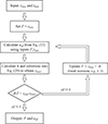 |
Figure 4 Iterative algorithm flowchart for effective radius calibration. |
This process ensures that the back-calculated z max and z min values based on the iteratively updated effective radius are consistent with the experimental observations, thereby enabling high-precision inversion of the transducer’s effective radius. This method does not rely on the direct measurement of the geometric focal length, making it applicable to transducers lacking focal length calibration data and enhancing the reliability of high-frequency focused acoustic field modeling.
2.1.2 Tone burst excitation mode
The theoretical models employed in this study are based on the acoustic field characteristics generated by the continuous-wave (CW) excitation of the transducers. Accordingly, equations (6), (7), and related expressions are derived under the assumption of CW excitation. However, to facilitate acoustic field measurements and mitigate the risk of potential damage to high-frequency transducers under prolonged CW excitation, experimental studies typically adopt tone-burst excitation instead of true continuous waves. Burst waves, also referred to as “quasi-continuous waves”, are distinct from pulse excitations because they consist of multiple sinusoidal cycles with a defined envelope. A schematic illustration of the burst waveform is shown in Figure 5.
 |
Figure 5 Waveform generated by tone burst excitation of the focusing transducer. (a) Tone burst. (b) Steady state. |
When a focusing transducer is driven by burst excitation, the radiated acoustic field can be regarded as a modulated wave train composed of a series of pulses. As this wave propagates to any spatial location, it generates a transient response signal resulting from the superposition of multiple acoustic pulses that arrive sequentially. Assuming that the vibration velocity across the radiating surface of the transducer is temporally synchronized (i.e., the vibration mode exhibits spatial uniformity), the contributions of different regions to the overall signal can be analyzed using the acoustic pressure waveform measured at the observation point. Typically, the leading edge of the signal is dominated by the direct wave emitted from the central region of the transducer, whereas the trailing edge is mainly influenced by edge waves radiating from the transducer’s periphery. In the intermediate portion of the signal, the pulses overlap to form a quasi-steady-state region, where the acoustic pressure amplitude remains relatively stable, as shown in Figure 5. Under these conditions, neglecting nonlinear distortion effects, the acoustic pressure amplitude at the field point exhibits an approximately linear relationship with the excitation voltage amplitude applied to the transducer. This steady-state signal can thus be considered a good approximation of the acoustic field distribution under continuous-wave (CW) excitation and is particularly suitable for representing the steady-state response of high-frequency transducers driven by CW signals.
Because the theoretical model calculates the acoustic pressure through surface integration over the transducer’s effective emission area, the integral outcome can only accurately represent the spatial acoustic pressure distribution when the individual pulses emitted by the transducer sufficiently overlap in the time domain and reach a stable superposition. Therefore, in the experiments, it is necessary to ensure that the burst excitation duration is sufficiently long to capture the complete acoustic pressure response in the steady-state region at the measurement point. The tone-burst excitation duration (denoted as τ in Fig. 5) determines the number of cycles in the excitation signal. To obtain a valid steady-state response, this duration should include at least several complete cycles, typically no fewer than 3 to 5, to guarantee that coherent superposition conditions are met as the acoustic field propagates to each spatial location. Additionally, the pulse repetition frequency (PRF) of the burst excitation must be appropriately set with an upper limit to avoid interference from reciprocal reflections in the measurements.
2.2 Acoustic pressure distribution in the focal plane
The acoustic characteristics at the focal plane of a focusing transducer represent key parameters for evaluating its performance. Within the focal plane of the focusing transducer, the spatial coordinates satisfy rcosθ = F and rsinθ = x. Similarly, by applying Fresnel approximation, the average acoustic pressure measured by the hydrophone in the focal plane can be expressed as:
 (21)
(21)
Figure 6 shows the lateral acoustic pressure distributions of the focusing transducers in the focal plane, calculated and compared using needle hydrophones with different diameters. The focusing transducers selected are the same as those used in the above simulations: 30 MHz and 75 MHz transducers.
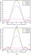 |
Figure 6 Lateral acoustic pressure distributions in the focal plane of the focusing transducers. (a) Focusing transducer at 30 MHz (nominal radius 0.125 inch). (b) Focusing transducer at 75 MHz (nominal radius 3 mm). |
It can be observed that the non-negligible spatial averaging effect of hydrophones in high-frequency acoustic field measurements primarily manifests as a systematic underestimation of the acoustic pressure amplitude and overestimation of the beamwidth in the focal plane. This effect stems from the finite size of the hydrophone’s sensitive surface: when its dimensions are comparable to or larger than the cross-sectional area of the sound beam, the recorded signal represents a spatially averaged acoustic pressure over the sensitive region, significantly reducing the hydrophone’s ability to resolve fine structures within the actual acoustic field distribution.
By comparing the measurement results obtained using an ideal-point receiver model with those from a real hydrophone of a finite aperture in the same transducer focal plane, the −6 dB beamwidth of high-frequency transducers can be accurately determined. In conjunction with the calibration of the effective radius, this approach yields acoustic field parameters that offer a more accurate representation of real-world conditions relative to relying on the transducer’s nominal parameters, thereby providing a more reliable basis and technical support for applications such as high-resolution ultrasonic nondestructive testing and material microstructure imaging.
2.3 Acoustic pressure distribution of focusing transducers in attenuating media
Up to here, this analysis was conducted under the assumption of negligible attenuation in the propagation medium. When considering attenuation, the wave number k can be replaced by a complex wave number k c :
 (22)
(22)
where the imaginary part α represents the acoustic attenuation coefficient of the medium, which exhibits a quadratic frequency dependence in liquid media (e.g., water), with units of dB/(m⋅MHz2).
For ultrasonic transducers excited by continuous-wave (CW) or burst signals, the operating frequency is typically a single frequency point. Therefore, in the theoretical derivation, a complex wave vector can first be adopted for the generalized treatment, where k c is explicitly expressed at the final calculation stage to quantify the influence of acoustic attenuation on the acoustic pressure distribution. Specifically, in equation (6), which describes the on-axis acoustic pressure distribution of the focusing transducers; and equation (21), which describes the lateral acoustic pressure distribution in the focal plane, the original wave number k is replaced by the complex wave vector k c . This substitution retains the mathematical structure of the original formulations while enabling the parametric analysis of attenuation effects in subsequent numerical simulations.
Figure 7 illustrates the variations in the on-axis and focal plane acoustic pressure distributions of a focusing transducer under different acoustic attenuation coefficients α. The transmitting transducer used is the previously mentioned V375, which has a nominal radius of 0.125 inch and a nominal focal length of 0.75 inch. As shown in Figure 2bluea, when the axial acoustic pressure is measured using a hydrophone with a 0.2 mm diameter, the amplitude difference between the minimum and maximum acoustic pressures is already significantly reduced, indicating a pronounced spatial averaging effect. Upon further consideration of the influence of acoustic attenuation, the fluctuation amplitude becomes even weaker and may become indistinguishable. Therefore, a needle hydrophone with a diameter of 40 μm is selected for the simulation to ensure a sufficient resolution.
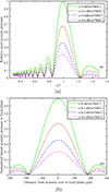 |
Figure 7 On-axis and focal plane acoustic pressure distributions of focusing transducer under various acoustic attenuation conditions. (a) On-axis acoustic pressure distribution. (b) Lateral acoustic pressure distribution in focus plane. |
Similar to the spatial averaging effect induced by hydrophones, acoustic attenuation in the propagation medium results in a reduction in the measured acoustic pressure amplitude. However, unlike the underestimation of the amplitude caused by spatial averaging, the attenuation-induced reduction in the amplitude reflects the actual physical loss of acoustic energy and therefore requires no correction. Further analysis of Figure 7 reveals that variations in the attenuation coefficient barely affect the spatial locations of the maximum and minimum acoustic pressure values along the acoustic axis, due to the very short focal length of the high-frequency focusing ultrasonic transducer. Similarly, in the focal plane, the positions of the acoustic pressure zero-crossing points remain unchanged, and the beamwidth is unaffected by acoustic attenuation. These observations indicate that, under the current theoretical model, acoustic attenuation primarily influences the amplitude of the acoustic pressure field rather than its spatial distribution characteristics. This outcome arises from the Fresnel approximation, which uniformly replaces the exact distance r′ from each radiating point to the receiving point with geometric focal length F in the integral term.
3 Experimental result
The system used to calibrate the effective parameters of the focusing ultrasonic transducer is shown in Figure 8. In this system, a computer interface with a motor control unit drives a three-axis stepper motor stage, enabling the three-dimensional scanning of the acoustic field. A needle hydrophone was fixed at a designated position to receive the ultrasonic signals radiated by the transducer. During the experiment, a sinusoidal burst signal was generated using a signal generator (Agilent Technologies 81150A) to excite the focusing transducer. An appropriate number of excitation cycles was selected to approximate the continuous-wave (CW) excitation, as assumed in the theoretical model. Ultrasonic signals were acquired using a Tektronix MDO34 digital oscilloscope, featuring a maximum sampling rate of 2.5 GSa/s and a bandwidth of 500 MHz. To minimize the significant spatial averaging effect in high-frequency acoustic field measurements, a 40 μm diameter needle hydrophone (SN253) manufactured by Precision Acoustics (UK) was employed as the receiver.
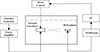 |
Figure 8 Schematic diagram of the acoustic field scanning system. |
3.1 Frequency measurement
Before calibrating the effective acoustic parameters of a focusing ultrasonic transducer, it is essential to calibrate its actual operating frequency to select an appropriate frequency for burst excitation. Because a piezoelectric transducer functions as a damped oscillatory system with inherent resonant characteristics [28], it is capable of responding to excitation signals over a certain frequency range. To comprehensively evaluate the acoustic response of the transducer across different frequency components, broadband pulse excitation was employed. In this study, a focusing piezoelectric transducer (NIM) with a nominal center frequency of 70 MHz was selected. The time-domain acoustic signal was acquired at the focal point of the transducer, and its frequency spectrum was obtained via Fourier transform. The resulting spectral distribution is shown in Figure 9.
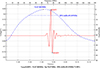 |
Figure 9 Time-frequency analysis of a 70 MHz focusing transducer at the focal point under pulse excitation. |
Spectral analysis confirmed that the dominant response frequency (i.e., center frequency) within the focal region under broadband excitation closely corresponded to the nominal frequency of the transducer. Consequently, in subsequent calibration procedures, burst signals centered at this frequency are employed as the excitation source to enhance the signal-to-noise ratio and facilitate a more accurate characterization of the spatial acoustic pressure distribution.
Although the transducer’s nominal center frequency is 70 MHz, the thickness-mode resonant frequency of its internal piezoelectric ceramic element is typically higher. The approximate relationship between the resonant frequency and thickness is given by
 (23)
(23)
where f is the thickness-mode resonant frequency, v is the longitudinal wave velocity of the material in the thickness direction, and d is the thickness of the piezoelectric plate. When ultrasonic waves propagate through a medium, high-frequency components are more strongly attenuated owing to frequency-dependent absorption. This results in a downward shift of the spectral centroid during propagation, causing the measured center frequency to be lower than the actual resonant frequency along with a certain degree of frequency bandwidth broadening.
Although broadband pulse excitation has been widely utilized in high-resolution ultrasonic nondestructive testing, ultrasonic microscopy, and related fields, the spatial distribution characteristics of the acoustic field generated by focusing transducers under such excitation conditions have not been widely studied. In particular, under non-steady-state broadband excitation, it is challenging to accurately characterize the effective acoustic parameters of a transducer. Therefore, this study uniformly adopts burst excitation to enable a clearer analysis of the transducer’s acoustic characteristics near the center frequency. This approach provides a more reliable experimental foundation for the extraction of effective acoustic parameters and modeling of focused acoustic fields.
3.2 On-axis measurement
Before performing axial scanning, it is crucial to ensure precise alignment between the central axis of the focusing transducer and hydrophone. Therefore, the scanning path must be carefully inspected and adjusted prior to digitizing and storing waveform data. At the beginning of each axial scan, preliminary alignment of the transducer and hydrophone is conducted in the post-focal range, followed by fine adjustments during the scanning process [29–31]. Ideally, the beam profile should remain perfectly symmetrical, obviating the need for further alignment correction. However, in practice, minor adjustments are occasionally necessary to maintain the measurement accuracy.
When scanning the on-axis acoustic pressure distribution in the pre-focal range, the waveform recorded by the oscilloscope deviated significantly from a sinusoidal pulse train with uniform amplitudes and exhibited notable morphological changes. As previously analyzed, the central portion of the waveform arises from the coherent cancellation of signals, representing the integral of the acoustic pressure contributions from each point on the transducer surface, as described in the theoretical model. This phenomenon is illustrated by the signal acquired in the pre-focal range region using a 30 MHz focusing transducer (V375, Olympus), as shown in Figure 10. Therefore, prior to further processing, it is necessary to truncate the on-axis acoustic pressure signal appropriately to extract the stable components contained within it.
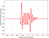 |
Figure 10 Pressure waveform of the transducer acquired in the pre-focal range by the oscilloscope. |
In this study, focusing transducers operating at four representative frequencies within the 30–100 MHz range, commonly used in high-frequency nondestructive testing and ultrasonic microscopy, were selected to verify the feasibility and effectiveness of the proposed theory. In particular, Figure 11 shows the following:
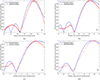 |
Figure 11 Measurement of on-axis acoustic pressure distribution for different focusing transducers. (a) 30 MHz focusing transducer. (b) 50 MHz focusing transducer. (c) 75 MHz focusing transducer. (d) 100 MHz focusing transducer. |
-
(a)
A 30 MHz focusing transducer with a nominal radius of 3.18 mm and nominal focal length of 19.05 mm (Olympus, V375);
-
(b)
A 50 MHz focusing transducer with a nominal radius of 3 mm and nominal focal length of 12 mm (NIM, NO. 4546346);
-
(c)
A 75 MHz focusing transducer with a nominal radius of 2 mm and nominal focal length of 12 mm (NIM, NO. 4550377);
-
(d)
A 100 MHz focusing transducer with a nominal radius of 2 mm and nominal focal length of 8 mm (NIM, NO. 4547473);
According to the experimental results presented in Figure 11, the on-axis acoustic pressure distributions of the focusing ultrasonic transducers at various frequencies, as measured by hydrophones, enabled the accurate identification of the maximum point z max and the minimum point z min. By integrating the theoretical framework described earlier with equation (13), an iterative algorithm was implemented in MATLAB to inversely calibrate the geometric focal length F, thereby allowing calculation of the transducer’s calibrated effective radius a eff. In the simulation section, the iteratively obtained values of F and a eff were used as inputs to generate the theoretical prediction curves (shown as blue solid lines). The results demonstrate a good agreement between the experimental measurements and theoretical simulations near the focal region, confirming the reliability and applicability of the proposed inversion method within this zone. However, the degree of agreement diminished at positions farther from the focus. This discrepancy can be primarily attributed to the following factors:
-
(1)
At positions far from the focal region, the signal amplitude becomes low, resulting in a poor signal-to-noise ratio (SNR), making the measurements vulnerable to environmental noise interference.
-
(2)
The acoustic beam generated by high-frequency focusing transducers is extremely narrow, and axial positioning errors have a pronounced impact on the acoustic pressure far from the focal region, even slight deviations can introduce significant measurement errors.
-
(3)
Systematic errors may arise from limitations in the hydrophone positioning accuracy and scanning step size.
-
(4)
A deviation of the real transducer from the radial symmetry assumed in the theory. Such deviation may disturb the on-axis pressure minima.
Table 1 summarizes the geometric focal lengths F and effective radii aeff calibrated via experimental iteration and inversion for each transducer across different frequencies and compares them with the nominal radius a specified by the manufacturer. It is evident that, under high-frequency operating conditions, the effective radius of the focusing transducers is generally smaller than their nominal values, which demonstrates a consistent trend across multiple frequency bands. Such discrepancies can result in substantial differences between the experimentally measured beamwidths and theoretical predictions, which must not be overlooked. To validate the accuracy and applicability of the calibrated effective radius aeff, subsequent experiments measure the −6 dB beamwidth in the focal plane and compared it with the theoretical acoustic field distribution after applying the calibration.
Analysis of on-axis acoustic pressure measurement results for different focusing transducers using a 40 μm hydrophone.
3.3 Focal plane measurement
This section investigates the acoustic pressure distribution characteristics of the transducers in the focal plane. The transducers mentioned above were used, and the scanning results are shown in Figures 12–15.
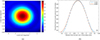 |
Figure 12 Scanning results of 30 MHz transducer using a 40 μm diameter needle hydrophone. (a) Field visualization in focal plane. (b) Pressure distribution in focal plane. |
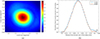 |
Figure 13 Scanning results of 50 MHz transducer using a 40 μm diameter needle hydrophone. (a) Field visualization in focal plane. (b) Pressure distribution in focal plane. |
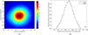 |
Figure 14 Scanning results of 75 MHz transducer using a 40 μm diameter needle hydrophone. (a) Field visualization in focal plane. (b) Pressure distribution in focal plane. |
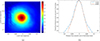 |
Figure 15 Scanning results of 100 MHz transducer using a 40 μm diameter needle hydrophone. (a) Field visualization in focal plane. (b) Pressure distribution in focal plane. |
Based on the aforementioned theory, the spatial averaging effect theoretical models for the axial and focal plane of the focusing transducers can fully reconstruct the true acoustic field distribution. To verify the effectiveness of the calibration, we performed theoretical calculations of the transducer’s acoustic field distribution under three different parameter settings and systematically compared them with the experimental measurements, as detailed in Table 2. The three comparison schemes are as follows:
Comparison of −6 dB beamwidth for different focusing transducers under three parameter schemes.
-
(a)
Using only manufacturer-provided nominal parameters: Acoustic field simulations were performed using the nominal focal length and transducer radius as specified by the manufacturer.
-
(b)
Calibrating only the focal length F: The effective radius a eff remained set to the nominal value, whereas the focal length was corrected based on the experimental results.
-
(c)
Simultaneously calibration of both F and a eff: The experimentally derived true values of the focal length and effective radius were both incorporated into the theoretical model for full calibration.
From the results presented in Table 2, it is evident that directly using the nominal parameters marked on the transducer housing for acoustic field modeling results in significant discrepancies between the theoretical calculations and experimental measurements. The error between the simulated and measured acoustic fields can be effectively reduced by experimentally measuring the on-axis acoustic pressure distribution and iteratively calibrating geometric focal length F. As shown in Table 2, this calibration decreases the relative error by approximately 50% compared with the uncalibrated model, significantly enhancing the prediction accuracy. Further calibration of the transducer’s effective radius a eff yields additional improvements in the simulation accuracy. Specifically, after the simultaneous calibration of both parameters, the relative error in the −6 dB beamwidth is reduced to within 3%, demonstrating a strong agreement between the theoretical model and experimental data. This confirms the effectiveness and reliability of the spatial averaging and parameter inversion approaches. This deviation may be attributed to the relatively high background noise during hydrophone scanning, which increases the uncertainty in sound pressure measurements, thereby affecting the measurement accuracy of the effective radius and focal length of the focusing transducer, ultimately resulting in errors in acoustic field calculations.
As discussed earlier, the spatial averaging effects become more pronounced with increasing hydrophone diameter. Therefore, selecting a hydrophone with a small sensitive element size that matches the beamwidth is crucial for ensuring the measurement accuracy during high-frequency transducer calibration. By combining the calibrated transducer parameters with the spatial averaging correction model presented in this study, real-time correction of acoustic pressure measurements during scanning is achievable, significantly enhancing the accuracy of the acoustic field reconstruction. This provides a more robust theoretical and experimental basis for the performance characterization and application of high-frequency focusing transducers.
4 Conclusion
The characterization of the acoustic field of focusing transducers operating at tens of megahertz remains a challenge due to the combined effects of low signal-to-noise ratio, high attenuation and highly focused directivity. A substantial body of prior research has primarily relied on theoretical models with limited experimental validation against actual transducer performance, thereby largely confining calibration efforts to low-frequency transducers.
To address the technical challenges in determining the acoustic field parameters of high-frequency focusing ultrasonic transducers, this study adopted a method that integrates theoretical modeling with experimental calibration. A sound field distribution model was established based on the Rayleigh integral, and the key parameters were inverted using hydrophone measurement data. The results indicated that the effective radius of high-frequency focusing transducers is generally smaller than the nominal value, and the direct application of nominal parameters can lead to calculation errors exceeding 10% in the −6 dB beamwidth. In contrast to studies that were confined to single-parameter calibration, this study simultaneously calibrated the geometric focal length F and effective radius aeff using an iterative algorithm. The size of the hydrophone significantly affects the spatial averaging effect, and a 40 μm needle hydrophone effectively reduces measurement distortion. In comparison with prior studies, the present study takes into account the combined influence of the transducer’s effective radius and the hydrophone’s spatial averaging effect. The errors between the measured and theoretical beamwidth values can be reduced to within 3%, significantly enhancing the accuracy of the acoustic field parameter characterization. This approach offers critical technical support for optimizing the design of high-frequency ultrasonic testing systems and the development of imaging algorithms, which is of great importance for precise micro-defect detection in aerospace, microelectronics, and other advanced fields. Future work may extend this methodology to acoustic field modeling and parameter calibration under broadband pulse excitation, further advancing the engineering applications of high-frequency focusing ultrasonic technology.
Funding
The authors would like to acknowledge the funding and support of the National Key R&D Program of China (2022YFF0706505), the National Natural Science Foundation of China (NSFC) (11904347), the Fundamental Research Funds of National Institute of Metrology (AKYZD2401) and the NMPA Key Laboratory for Quality Evaluation of Ultrasonic Surgical Equipment.
Conflicts of interest
The authors declare that they do not have any conflict of interest.
Data availability statement
Data are available on request from the authors.
References
- G. D’Angelo, S. Rampone: Feature extraction and soft computing methods for aerospace structure defect classification. Measurement 85 (2016) 192–209. [Google Scholar]
- M. Silva, E. Malitckii, T. Santos, P. Vilaça: Review of conventional and advanced non-destructive testing techniques for detection and characterization of small-scale defects. Progress in Materials Science 138 (2023) 101155. [Google Scholar]
- A. Zarei, S. Pilla: Laser ultrasonics for nondestructive testing of composite materials and structures: a review. Ultrasonics 136 (2024) 107163. [Google Scholar]
- B. Wang, S. Zhong,T.-L. Lee, K.S. Fancey, J. Mi: Non-destructive testing and evaluation of composite materials/structures: a state-of-the-art review. Advances in Mechanical Engineering 12, 4 (2014) 1687814020913761. [Google Scholar]
- S. Gholizadeh: A review of non-destructive testing methods of composite materials. Procedia Structural Integrity 1 (2016) 50–57. [Google Scholar]
- K. Ali, A. Abdalla, D. Rifai, M. Faraj: A review on system development in eddy current testing and technique for defect classification and characterization. IET Circuits, Devices & Systems 11, 4 (2017) 330–343. [Google Scholar]
- D. Zhang, W. Jackson, G. Dobie, C. Macleod, A. Gachagan: Innovative non-invasive ultrasound method for whisky cask liquid level measurement. Measurement 228 (2024) 114345. [Google Scholar]
- F. Qian, G. Xing, P. Yang, P. Hu, L. Zou, T. Koukoulas: Laser-induced ultrasonic measurements for the detection and reconstruction of surface defects. Acta Acustica 5 (2021) 38. [CrossRef] [EDP Sciences] [Google Scholar]
- L. Qin, Y. Lu, Y. Xu, W. He: The calibration methods of hydrophones for underwater environmental sound measurements or biomedical ultrasound measurements: a review. Measurement 242, A (2025) 115700. [Google Scholar]
- ASTM International: ASTM E1065/E1065M-14, Standard Guide for Evaluating Characteristics of Ultrasonic Search Units. ASTM International, West Conshohocken, PA, 2014. [Google Scholar]
- ISO 16811: Non-destructive testing – Ultrasonic testing – Characterization of search unit and sound field. International Organization for Standardization, Geneva, Switzerland, 2012. [Google Scholar]
- Y. Ping, X. Guangzhen, H. Longbiao: Calibration of high-frequency hydrophone up to 40 MHz by heterodyne interferometer. Ultrasonics 54 (2014) 402–407. [Google Scholar]
- X. Guangzhen, Y. Ping, H. Longbiao, F. Xiujuan: Spatial averaging effects of hydrophone on field characterization of planar transducer using Fresnel approximation. Ultrasonics 71 (2016) 51–58. [Google Scholar]
- G. Xing, P. Yang, P. Hu, K.H. Lam, L. He, Z. Zhang: Field characterization of steady state focused transducers using hydrophones based on Fresnel approximation. Measurement Science and Technology 28 (2017) 065005. [Google Scholar]
- M. Weber, V. Wilkens: A comparison of different calibration techniques for hydrophones used in medical ultrasonic field measurement. IEEE Transactions on Ultrasonics, Ferroelectrics, and Frequency Control 68, 5 (2021) 1919–1929. [Google Scholar]
- F.S. Foster, G.R. Lockwood, L.K. Ryan, K.A. Harasiewicz, L. Berube, A.M. Rauth: Principles and applications of ultrasound backscatter microscopy. IEEE Transactions on Ultrasonics, Ferroelectrics, and Frequency Control 40, 5 (1993) 608–617. [Google Scholar]
- E. Martin, B. Treeby: Investigation of the repeatability and reproducibility of hydrophone measurements of medical ultrasound fields. Journal of the Acoustical Society of America 145, 3 (2019) 1270. [Google Scholar]
- E.G. Radulescu, P.A. Lewin, A. Goldstein, A. Nowicki: Hydrophone spatial averaging corrections from 1 to 40 MHz. IEEE Transactions on Ultrasonics, Ferroelectrics, and Frequency Control 48, 6 (2001) 1575–1580. [Google Scholar]
- B.A. Auld: Acoustic Fields and Waves in Solids, Vol. 1, 2nd ed. Krieger Publishing Company, Malabar, FL, 1990. [Google Scholar]
- Y. Wu: Measurement of effective radii of ultrasonic transducers [Ph.D. dissertation]. Philadelphia (PA): Drexel University, 1992. Order No. 30755041. [Google Scholar]
- S.M. Nagle, G. Sundar, M.E. Schafer, G.R. Harris, S. Vaezy, J.M. Gessert, S.M. Howard, M.K. Moore, R.M. Eaton: Challenges and regulatory considerations in the acoustic measurement of high-frequency (> 20 MHz) ultrasound. Journal of Ultrasound in Medicine 32, 11 (2013) 1897–1911. [Google Scholar]
- G.R. Harris, S.M. Howard, A.M. Hurrell, P.A. Lewin, M.E. Schafer, K.A. Wear, V. Wilkens, B. Zeqiri: Hydrophone measurement for biomedical ultrasound applications: a review. IEEE Transactions on Ultrasonics, Ferroelectrics, and Frequency Control 70, 2 (2023) 85–100. [Google Scholar]
- D. Cathignol, O.A. Sapozhnikov, J. Zhang: Lamb waves in piezoelectric focused radiator as a reason for discrepancy between O’Neil’s formula and experiment. Journal of the Acoustical Society of America 101, 3 (1997)1286–1297. [Google Scholar]
- L.E. Kinsler, A.R. Frey, A.B. Coppens, J.V. Sanders: Fundamentals of Acoustics, 4th ed. John Wiley & Sons, New York, 2000. [Google Scholar]
- M.S. Canney, M.R. Bailey, L.A. Crum, V.A. Khokhlova, O.A. Sapozhnikov: Acoustic characterization of high intensity focused ultrasound fields: a combined measurement and modeling approach. Journal of the Acoustical Society of America 124, 4 (2008) 2406–2420. [Google Scholar]
- O. Bessonova, V. Wilkens: Membrane hydrophone measurement and numerical simulation of HIFU fields up to developed shock regimes. IEEE Transactions on Ultrasonics, Ferroelectrics, and Frequency Control 60, 2 (2013) 290–300. [Google Scholar]
- H.T. O’Neil: Theory of focusing radiators. Journal of the Acoustical Society of America 21, 5 (1949) 516–526. [Google Scholar]
- S.O.R. Moheimani, A.J. Fleming: Piezoelectric Transducers for Vibration Control and Damping. Springer, 2006. [Google Scholar]
- J. Adach, R.C. Olivers: A detailed investigation of effective geometrical parameters for weakly focused ultrasonic transducers. Part I: optimization of experimental procedures. Acta Acustica 70, 1 (1990) 12–22. [Google Scholar]
- J. Adach, R.C. Chivers: A detailed investigation of effective geometrical parameters for weakly focussed ultrasonic transducers. Part II: A systematic study including an absorbing medium. Acta Acustica 70, 2 (1990) 135–145. [Google Scholar]
- R.C. Preston, D.R. Bacon, R.A. Smith: Calibration of medical ultrasonic equipment-procedures and accuracy assessment. IEEE Transactions on Ultrasonics, Ferroelectrics, and Frequency Control 35, 2 (1988) 110–121. [Google Scholar]
Cite this article as: Lu H. Xing G. Yang P. Qian F. Wang K. He L. & Hu J. 2025. Determination of acoustic field parameters for high-frequency focusing ultrasonic transducers up to 100 MHz. Acta Acustica, 9, 67. https://doi.org/10.1051/aacus/2025052.
All Tables
Analysis of on-axis acoustic pressure measurement results for different focusing transducers using a 40 μm hydrophone.
Comparison of −6 dB beamwidth for different focusing transducers under three parameter schemes.
All Figures
|
Figure 1 Measurement of the acoustic field of a focusing transducer using a needle hydrophone. |
| In the text | |
|
Figure 2 On-axis acoustic pressure distribution of focusing transducers measured by different hydrophones. (a) Focusing transducer at 30 MHz (nominal radius 0.125 inch). (b) Focusing transducer at 75 MHz (nominal radius 3 mm). |
| In the text | |
|
Figure 3 Schematic diagram of geometric structure of focusing transducer. |
| In the text | |
|
Figure 4 Iterative algorithm flowchart for effective radius calibration. |
| In the text | |
|
Figure 5 Waveform generated by tone burst excitation of the focusing transducer. (a) Tone burst. (b) Steady state. |
| In the text | |
|
Figure 6 Lateral acoustic pressure distributions in the focal plane of the focusing transducers. (a) Focusing transducer at 30 MHz (nominal radius 0.125 inch). (b) Focusing transducer at 75 MHz (nominal radius 3 mm). |
| In the text | |
|
Figure 7 On-axis and focal plane acoustic pressure distributions of focusing transducer under various acoustic attenuation conditions. (a) On-axis acoustic pressure distribution. (b) Lateral acoustic pressure distribution in focus plane. |
| In the text | |
|
Figure 8 Schematic diagram of the acoustic field scanning system. |
| In the text | |
|
Figure 9 Time-frequency analysis of a 70 MHz focusing transducer at the focal point under pulse excitation. |
| In the text | |
|
Figure 10 Pressure waveform of the transducer acquired in the pre-focal range by the oscilloscope. |
| In the text | |
|
Figure 11 Measurement of on-axis acoustic pressure distribution for different focusing transducers. (a) 30 MHz focusing transducer. (b) 50 MHz focusing transducer. (c) 75 MHz focusing transducer. (d) 100 MHz focusing transducer. |
| In the text | |
|
Figure 12 Scanning results of 30 MHz transducer using a 40 μm diameter needle hydrophone. (a) Field visualization in focal plane. (b) Pressure distribution in focal plane. |
| In the text | |
|
Figure 13 Scanning results of 50 MHz transducer using a 40 μm diameter needle hydrophone. (a) Field visualization in focal plane. (b) Pressure distribution in focal plane. |
| In the text | |
|
Figure 14 Scanning results of 75 MHz transducer using a 40 μm diameter needle hydrophone. (a) Field visualization in focal plane. (b) Pressure distribution in focal plane. |
| In the text | |
|
Figure 15 Scanning results of 100 MHz transducer using a 40 μm diameter needle hydrophone. (a) Field visualization in focal plane. (b) Pressure distribution in focal plane. |
| In the text | |
Current usage metrics show cumulative count of Article Views (full-text article views including HTML views, PDF and ePub downloads, according to the available data) and Abstracts Views on Vision4Press platform.
Data correspond to usage on the plateform after 2015. The current usage metrics is available 48-96 hours after online publication and is updated daily on week days.
Initial download of the metrics may take a while.