| Issue |
Acta Acust.
Volume 9, 2025
|
|
|---|---|---|
| Article Number | 69 | |
| Number of page(s) | 13 | |
| Section | Environmental Noise | |
| DOI | https://doi.org/10.1051/aacus/2025053 | |
| Published online | 18 November 2025 | |
Scientific Article
Atmospheric turbulence affects noise annoyance from aircraft flyovers
Empa, Swiss Federal Laboratories for Materials Science and Technology, Dübendorf, Switzerland
* Corresponding author: This email address is being protected from spambots. You need JavaScript enabled to view it.
Received:
22
June
2025
Accepted:
5
October
2025
Abstract
Auralization of outdoor sound propagation has become an important tool for studying noise perception in the contexts of aircraft, wind farm, and drone noise. To achieve high realism, these auralizations consider amplitude fluctuations caused by atmospheric turbulence. In a recent publication, a semi-empirical model was introduced which is applicable to relatively long outdoor sound propagation such as aircraft and wind farm noise, as it considers the saturation effect for amplitude fluctuations in the partially-saturated regime. This article presents a study applying the semi-empirical model for investigating the impact of turbulence-induced amplitude fluctuations on annoyance in auralized aircraft flyovers. For this, two 2-alternative-forced-choice listening experiments were conducted in a controlled laboratory setting: the first tested whether participants could reliably detect audible differences between aircraft flyovers under different meteorological conditions; the second assessed which condition was perceived as more annoying. The results show that strong differences in meteorological conditions and the respective atmospheric turbulence can lead to salient audible differences. Relative annoyance ratings tend to increase with stronger atmospheric turbulence. Further, the data suggest that amplitude fluctuations can interact with other characteristics of aircraft noise such as fan tones and alter the perceptual impact of these characteristics. Therefore, the study highlights the importance of modeling turbulence-induced amplitude fluctuations in realistic aircraft auralizations, and presumably also wind farm and drone noise auralization, as the perceptual impression can be affected in several ways.
Key words: Aircraft noise auralization / Atmospheric turbulence / 2-AFC listening experiments / Noise annoyance / Outdoor sound propagation
© The Author(s), Published by EDP Sciences, 2025
 This is an Open Access article distributed under the terms of the Creative Commons Attribution License (https://creativecommons.org/licenses/by/4.0), which permits unrestricted use, distribution, and reproduction in any medium, provided the original work is properly cited.
1 Introduction
Auralization of outdoor sound propagation under realistic atmospheric conditions has become an important tool for studying noise perception in the contexts of aircraft, wind farm, and drone noise. Realistic modeling of the atmosphere includes sound scattering by turbulence, which induces fluctuations in sound amplitude and phase, known as acoustic scintillations, resulting in audible amplitude modulations and randomized phase shifts [1, 2].
Recent auralization methods account for turbulence-induced amplitude fluctuations using theoretical models developed by Ostashev and Wilson [3], which describe amplitude and phase fluctuations in the weak-scattering regime (i.e., short propagation distances and weak turbulence). These models have been validated within their range of applicability [4, 5]. Building on this framework, Bresciani et al. [6] proposed an auralization method that synthesizes acoustic scintillation sequences using spatial correlation functions of log-amplitude and phase fluctuations. This work extends earlier efforts [7], which relied on simplified turbulence models [8]. The method was then applied to wind farm noise auralization [9]. Similarly, Prescher et al. [10] adapted these formulations for frequency-domain auralization of aircraft noise. In a slightly different approach, Forssén [11] suggested a method, where both the decorrelation effect by randomized phase and the random amplitude fluctuations are recreated in a single process, while the before mentioned methods use separate processes for phase and amplitude.
However, the theoretical model by Ostashev and Wilson does not capture the saturation of log-amplitude fluctuations that occurs in partially-saturated and strong scattering regimes, which are relevant for longer propagation distances in the atmosphere [1]. The existing auralization methods attempt to correct for this limitation using fixed upper limits or theoretical approximations, which remain relatively coarse.
To address this, we recently presented an empirical study on the saturation of log-amplitude fluctuations in aircraft flyover noise and proposed a semi-empirical model that predicts partially saturated fluctuations based on meteorological conditions and propagation distance [12]. This model has been integrated into a validated aircraft noise auralization framework [13], enabling more realistic representations of turbulence effects.
The enhanced auralization method makes it possible to study the effect of turbulence-induced noise fluctuations in perceptual studies. Prior research has shown that amplitude modulations in broadband noise can increase annoyance, especially when the modulations are random or of greater depth [14–16]. These findings suggest that different meteorological conditions and the resulting variations in atmospheric turbulence may significantly affect perceived aircraft noise annoyance.
This article presents a study investigating the impact of turbulence-induced amplitude fluctuations on annoyance in auralized aircraft flyovers. The analysis seeks to answer the research question Does the difference in turbulence between the two aircraft flyovers predict which is judged as more annoying? For this, the proposed auralization filters for modeling coherence loss in ground effect [17] and turbulence-induced amplitude fluctuations [12] are refined to reflect the latest state-of-the-art in turbulence modeling. The turbulence filters are applied to aircraft auralizations, which have been validated and analyzed for plausibility in a previous study [18]. Two listening experiments were conducted: the first tested whether participants could reliably detect audible differences between flyovers under different meteorological conditions; the second assessed which condition was perceived as more annoying. Annoyance responses were analyzed using generalized linear mixed models with the relative turbulence differences as well as the aircraft type as fixed effects and random intercepts for participants to account for repeatedmeasures.
The paper is structured as follows: Section 2 revisits the turbulence modeling approaches. Section 3 provides details on the synthesis of aircraft flyovers, the meteorological scenarios, filter implementation, and the design of the listening experiments. Results are presented in Section 4, discussed in Section 5, and summarized in the conclusion (Sect. 6).
2 Turbulence modeling
2.1 Amplitude fluctuation
2.1.1 Semi-empirical model
In this study, a recent model for turbulent log-amplitude fluctuations, presented in [12], is applied. This model is a semi-empirical extension of a theoretical model [3], based on a large dataset of aircraft flyovers. Figure 1 shows the geometry of the modeled sound source at height hs moving above a receiver at height hr with distance L.
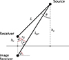 |
Figure 1. Geometry of aircraft flyover. |
The semi-empirical model introduces five modifications compared to the theoretical model. The modifications and its relevance because of the given meteorological conditions are briefly summarized in thefollowing:
-
(1)
Turbulence decay time is considered for meteorological conditions with decreasing intensity of the sun, which leads to a faster decrease of the surface sensible heat flux Q H compared to the the boundary layer height z i and the turbulent kinetic energy in the boundary layer. If the condition
 is true, the value for Q
H
is replaced by Q
H
(t − 3t
*), where t
* = z
i
/w
* is the turbulence decay time [19] and w
* is the convection velocityscale.
is true, the value for Q
H
is replaced by Q
H
(t − 3t
*), where t
* = z
i
/w
* is the turbulence decay time [19] and w
* is the convection velocityscale. -
(2)
Buoyancy-produced velocity fluctuations are neglected in stable boundary layers. This modification is applied if the surface sensible heat flux Q H is below zero, indicating a stable boundary layer suppressing turbulence.
-
(3)
Turbulence production by low level jets is approximated. This modification does apply if the condition 0.1u 100 m > 3u * is met, where u 100 m is the wind speed at 100 m height and u * is the friction velocity.
-
(4)
The propagation distance is replaced by an effective propagation distance L eff, which accounts for the fact, that the altitude of aircraft during takeoff and landing can often exceed the boundary layer height, while kinetic energy is much lower above the boundary layer than within. The effective propagation distance is then determined by:
 (1)
(1)
where L ABL is the sound propagation distance within the atmospheric boundary layer (ABL).
-
(5)
Partial saturation of amplitude fluctuations is considered. Section 2.1.2 presents the representation of log-amplitude fluctuations that allows the determination of theoretical boundary between weak-scattering and strong-scattering regime.
2.1.2 Determination of the theoretical boundary between weak and strong-scattering regime
In the semi-empirical model, log-amplitude fluctuations  are described using the strength parameters Φ:
 (2)
(2)
Here, σ χ, T 2, σ χ, v s 2, and σ χ, v b 2 are the standard deviations of log-amplitude fluctuations due to fluctuations in temperature, shear-produced and buoyancy-produced wind velocity given by the theoretical model in [3] for weak-scattering regimes. Φ T, v s, v b 2 are the height-dependent strength parameters for fluctuations in temperature, shear-produced and buoyancy-produced wind velocity [12]:
 (3)
(3)
 (4)
(4)
Here, Γ(n)=(n − 1)! is the definition of the gamma function valid for positive integers, k is the acoustical wavenumber, T 0 is a reference temperature, c 0 the reference speed of sound, z is the integration variable in vertical direction. The ordinary von Kármán spectrum is obtained by setting α = 11/6. L T , L v s , and L v b are the length scales of temperature fluctuations and of shear-produced and buoyancy-produced wind velocity fluctuations [3].
The strength parameter Φ2 allows consideration of the theoretical boundary between the weak-scattering and the strong-scattering regime.
Φmax 2 is the maximum strength parameter in the weak-scattering regime [20]:
![Mathematical equation: $$ \begin{aligned} \mathrm {{\Phi }} _{\max }{^2}=\frac{2 b{^2}}{\begin{array}{c}\beta _T\left[1-H_T\left(D_T\right)\right]+\beta _{vs}\left[1-H_v\left(D_{vs}\right)\right] +\beta _{vb}\left[1-H_v\left(D_{vb}\right)\right]\end{array}}\cdot \end{aligned} $$](/articles/aacus/full_html/2025/01/aacus250084/aacus250084-eq7.gif) (5)
(5)
Here, b 2 is a coefficient representing the boundary between weak and strong scattering, which was empirically determined in [12] with b 2 = 1/6. The functions H T and H v describe the effect of diffraction on σ 2 [20]:
 (6)
(6)
 (7)
(7)
with the integration variable  where κ is the turbulence wavenumber and
  for direct sound propagation from an elevated source to an elevated receiver where h
s
≫ h
r
.
for direct sound propagation from an elevated source to an elevated receiver where h
s
≫ h
r
.
The height-dependent wave parameter D T, v for temperature and wind velocity fluctuations is given as [12]:
 (8)
(8)
The coefficients β T , β v s , and β v b are determined by the ratio of the strength parameters relative to the strongest strength parameter:
 (9)
(9)
For each point during the flyover, the lowest frequency (limit frequency f lim) which exceeds the theoretical boundary between weak-scattering and strong-scattering regime can be determined using the inequality
 (10)
(10)
Meteorological conditions of auralized aircraft flyover.
Overview of considered cases and limit frequency f lim (Hz) indicating the theoretical boundary between weak-scattering and strong-scattering regime for the moment of direct flyover.
2.2 Coherence factor
We presented a method to model coherence loss in ground effect by atmospheric turbulence for auralizations of aircraft flyovers measured with a single microphone in [17]. The method is based on the coherence factor C coh for horizontal sound propagation as described in [2]. In a more recent study [21], a formulation of the coherence factor for vertical and slanted sound propagation [3, 5] was applied to the modeling of coherence loss in a microphone array located at the ground. In the current study, the later formulation of the coherence factor for vertical and slanted sound propagation is used to auralize aircraft flyover over a single microphone.
The coherence factor for vertical and slanted line-of-sight propagation is given as
![Mathematical equation: $$ \begin{aligned} C_{\text{ coh}}(L ; r_d)&= \exp \left\{ -\frac{\pi ^{2} k_{0}^{2}}{\cos \theta } \int _{h_r}^{h_s} \,\mathrm{d}z \int _{0}^{\infty } \mathrm{\Phi }_{\mathrm{eff} }(z, \kappa )\right.\nonumber \\ &\quad \times \!\left. \left[1-J_{0}\left(\frac{\kappa z r_d}{h_s-h_r}\right)\right] \kappa \,\mathrm{d}\kappa \right\} , \end{aligned} $$](/articles/aacus/full_html/2025/01/aacus250084/aacus250084-eq15.gif) (11)
(11)
with L = (h s − h r )/cosθ, the sound path separation r d , k 0 = ω/c 0 the reference acoustical wavenumber in air for the reference sound speed c 0, J 0 is the Bessel function of the first kind and zero order, and Φeff is the effective turbulence spectrum. The sound path separation r d is determined as
 (12)
(12)
The definition of the effective turbulence spectrum Φeff can be found in [3, 21].
3 Method
In this section, it is shown how the turbulence modeling is integrated in the auralization process. The created samples for the listening experiment and the setup of the listening experiments will be described.
3.1 Synthesis of aircraft flyovers
For this study, flyovers of two current airliner types, i.e., an Airbus A320-214 and an A340-313, during departure are auralized considering different meteorological conditions. The synthesis method is described in [13, 18]. The emission and the flight path data have been used in a previous study [18]. Compared to this study, buzzsaw and fan tonal noise emissions are attenuated by 10 dB and 5 dB, respectively, in accordance with [12]. The receiver is located at h r = 10 m above grassy ground. During direct flyover, the Airbus A320 is at an altitude of h s = 700 m, the Airbus A340 is at an altitude of h s = 400 m.
The outdoor sound propagation modeling considers the effects of geometrical spreading, Doppler frequency shift, ground reflection, and air attenuation by models described in [13]. Additionally, the effects by atmospheric turbulence, i.e., coherence loss in ground effect and turbulent amplitude fluctuations are considered by using the models described in Section 2.
3.2 Atmospheric turbulence conditions
For both aircraft types, sound propagation is modeled for three different conditions of atmospheric turbulence. Table 1 gives the meteorological conditions and the time of the day. The conditions correspond to real-world meteorological conditions measured on two different days in July in Switzerland. The meteorological conditions are ranked into three turbulence categories: low, intermediate, and high.
In Table 2, the limit frequencies f
lim between weak-scattering and strong-scattering for the moment of direct flyover are given. For meteo condition C (cases III and VI), f
lim remains below 250 Hz during the whole flyovers. In these cases, log-amplitude fluctuations are clearly in the partially-saturated turbulence regime and thus strong turbulence effects are expected. In contrast, for case IV, the boundary to the strong-scattering regime is exceeded only for very high frequencies. This flyover is least affected by atmospheric turbulence. These different behaviors are illustrated in Figure 2 which shows the frequency dependency of the log-amplitude fluctuation  for four cases.
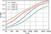 |
Figure 2. Frequency dependency of log-amplitude fluctuation |

3.3 Modeling turbulence effects in the auralization
This section explains how the influences of different atmospheric turbulence conditions on the synthesized aircraft sounds are realized in the auralization. The basis for this is the turbulence modeling in Section 2. Using these modeling results, a series of time-variant filters is designed to reproduce the turbulence effects on the sound pressure signals.
To model coherence loss in ground effect, the coherence factor C coh is used. C coh is computed with equation (11) at an update interval of 100 ms. C coh thus becomes a function of frequency f and time t. For each spectral C coh, a time-domain decorrelation filter is designed following the partial phase randomization approach in [17]. This approach was established specifically for the auralization of aircraft flyovers with signals composed of broadband noise and frequency-modulated tones. The filter is a time-varying finite impulse response (FIR) filter which is applied to either the direct sound, or the ground reflected sound signal. Its frequency response has the form [17]
![Mathematical equation: $$ \begin{aligned} B(f) = \text{ exp}\left( -j\phi (f) \left[ 1 - C_{\text{ coh}}(f,t)\right]^{2/3} \right), \end{aligned} $$](/articles/aacus/full_html/2025/01/aacus250084/aacus250084-eq19.gif) (13)
(13)
with the imaginary unit j and a random phases ϕ. The application of this filter leads to a partial loss of coherence between direct and ground reflected sound and thus reduces the prominence of the spectral ground effect pattern. Please note that this approach is not well suited for a single pure tone, i.e., a tone with constant frequency.
To model turbulent amplitude fluctuations, the semi-empirical model described in Section 2.1 is used. With this model, the log-amplitude fluctuation  is computed at an update interval of 200 ms. Using this time series, the effect of random amplitude fluctuations is implemented by a time-variant high shelving filter. In earlier work [13], we used a first-order high shelving filter for this. However, here we found that a first-order filter cannot reproduce the frequency dependency of the recently developed model by Lincke et al. [12]. The slopes of
  are in fact clearly lower than the ones used in [13] and cannot be realized using a first-order filter. Furthermore, we found that the slopes of
  vary between different meteorological conditions (see e.g., Fig. 2).
To overcome these limitations, here we propose to use a second-order high shelving filter which allows the shelf slope to be adjusted. The second order filter has a continuous-time prototype transfer function of the form
 (14)
(14)
with s = j
ω/ω
0, where ω = 2π
f is the angular frequency and ω
0 the angular frequency at mid-point of the filter slope. The amplitude A is related to the high frequency filter gain G (in dB) by A = 10
G/40. The quality factor Q is used to modify the shelf slope. A filter H
1 with a transfer function according to equation (14) is designed that matches its magnitude response to the  curve
curve
 (15)
(15)
by estimating the three parameters G, ω 0, and Q.
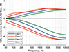 |
Figure 3. Statistical magnitude responses of amplitude modulation (AM) filters to reproduce turbulence-induced amplitude fluctuations for different cases. The curves show the upper and lower bounds of the 68% confidence bands at shortest distance of the aircraft. |
The filter equation (14) is realized in discrete-time by an infinite impulse response (IIR) filter. The filter coefficients are updated at audio sampling rate. This first IIR filter H 1 realizes the frequency dependent amplitude modulations. A second IIR filter H 2 is connected in cascade to ensure that overall energy neutrality is maintained. This energy correction filter has a frequency response
 (16)
(16)
assuming normally distributed level fluctuations. Figure 3 shows the magnitude responses of both filters combined in a statistical sense for the four cases from Figure 2. The confidence band limits in Figure 3 are asymmetric with respect to the 0 dB line. This asymmetry is a consequence of the enforced energy neutrality of the turbulence filtering.
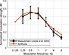 |
Figure 4. Modulation spectrum of level fluctuations in octave bands. Black curve indicated mean fluctuation of measurements presented in [12]. Error bars indicate standard deviation of measurements. Orange line represents modulation spectrum of synthesized fluctuations. |
The frequency-dependent amplitude fluctuations are introduced with the filter H 1 by varying its high frequency gain G 1 as a function of time. The resulting level fluctuations per frequency are shown in Figure 3 as the widths of the confidence bands. The modulation signal G1(t) is synthesized by filtering white Gaussian noise with a first-order low pass filter with a cutoff frequency of 0.5 Hz. Figure 4 compares the resulting modulation spectrum to measured data. The modulation strength is highest in the modulation frequency band of the 0.5 Hz octave. For illustration purposes, Figure 5 shows an example of resulting level fluctuations within a selected frequency band. For this example, the turbulence filters above described were designed for case I and applied to a pink noise signal. The obtained signal was sent through a 2 kHz octave band filter and analyzed as 100 ms short-term Leqs. The displayed level fluctuation signal, ΔL, is the difference between the Leqs and their mean value.
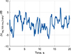 |
Figure 5. Generated level fluctuations for case I in the 2 kHz octave band. The standard deviation of this signal is 2.6 dB. |
Figures 6 and 7 present spectrograms of the resulting flyover auralizations. For the meteorological condition C (bottom figures), both flyovers exhibit a vertical pattern in the high frequency range indicating sudden amplitude fluctuations. Low frequencies are less affected and hardly exhibit a vertical pattern.
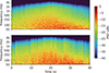 |
Figure 6. Spectrograms of auralized Airbus A320 in low and high turbulence conditions. Top: low turbulence condition A (case I); Bottom: high turbulence condition C (case III). |
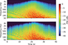 |
Figure 7. Spectrograms of auralized Airbus A340 in low and high meteorological turbulence conditions. Top: low turbulence condition A (case IV); Bottom: high turbulence condition C (case VI). |
The auralized aircraft flyovers for all meteorological conditions can be accessed under the reference [22]. In addition to the audio samples with turbulence filter, the auralizations without turbulence filtering are uploaded.
3.4 Listening experiments
3.4.1 General purpose and structure of experiments
The listening experiments were conducted in two stages. The first stage of the experiment focused on the distinguishability of fluctuations under different meteorological conditions. In this case, the null hypothesis stated that participants cannot perceive a difference between any combination of samples featuring different intensities of turbulence-induced amplitude fluctuations. To address the situation in which the first stage null hypothesis was rejected, a second experiment stage was planned to examine the influence of different meteorological conditions on the perception of annoyance.
To create the spatial auditory impression of a flyover in the listening experiment, the synthesized sound pressure signal was spatialized using a spherical loudspeaker array under controlled laboratory conditions. Empa’s listening test facility AuraLab in Switzerland was used.Participants received instructions and enterd their answers into software that they interacted with via a touchscreen. The sound pressure level of the reproduction was adjusted so that L AFmax remained below 75 dB(A). A detailed description of the test facility is given in Section 4.4 of [18].
Prior to starting the experiment, participants were provided study information in written form and were requested to sign a consent form for their participation. Following this, they entered the AuraLab, where they received further study information and instructions on the test software verbally. The duration of the experiments was approximately 10 min on average. The listening experiment was followed by a short questionnaire in which participants rated the difficulty of the task on a scale from 1 (very easy) to 5 (very difficult) and had space for comments. Participants completed the experiments individually, with no interaction with other participants. Participants were not compensated for their participation.
3.4.2 Experiment 1
In the first stage of the listening experiments, study participants did pairwise comparisons (two-alternative forced choices, 2-AFC) of synthesized aircraft flyovers with same or different conditions of atmospheric turbulence. Each sample was 20 s long. Participants were informed that only the meteorological condition could differ between the presented pair of samples. Participants were asked to state whether they were presented with two identical situations or with different ones. Playback could be repeated as often as desired but could not be interrupted once a sample started playing.
Participants had to assess seven comparisons. Only stimuli with meteo conditions A and C were included, with an additional sample without any applied turbulence filtering (called case 0). The presented pairs of cases are I vs III, III vs I, IV vs VI, VI vs IV, I vs I, IV vs IV, and IV vs 0.
All seven stimuli pairs were presented in individually randomized order for each participant. An odd number of pairs was intentionally selected to obscure any identifiable pattern in the presentation of the samples. In total, 12 expert listeners took part in the first stage of the experiment. The expert listeners were Empa Acoustics and Noise Control Laboratory employees, most of whom had prior experience of participating in experiments at the test facility.
3.4.3 Experiment 2
The second stage of the experiment was conducted independently of the first stage, two weeks later. The structure of the experiment was the same as in experiment 1. Study participants again did pairwise comparisons of synthesized aircraft flyover. Participants were asked to indicate which of two presented samples they found more annoying. Before the beginning of the experiment, the participants were given the following written instructions: In this experiment, you will listen to synthetic auralized aircraft flyovers. Each task presents you with two flyover samples for comparison. The aircraft and its trajectory remain the same in both samples – the only difference is the meteorological condition.
During the comparison, the following instruction was presented on the touchscreen: Imagine you are sitting at a peaceful outdoor location. Which sample do you find more annoying? Again, playback could be repeated as often as desired but could not be interrupted once a sample started playing. In this stage, all cases I to VI were included. Participants had to assess the pairwise comparison of all combinations of meteo conditions for each aircraft type, resulting into six comparisons. Each of the six stimulus pairs was evaluated once per participant. The order of the presented pairs and the order of the samples within a pair were randomized and varied across participants. In total, 29 individuals, 8 female and 21 male, participated in the second stage of the experiment. Of this, 12 can be considered expert listeners, 17 can be considered naive listeners. Participants were between 24 and 63 years old, with an average age of 38.
3.5 Data analysis
To determine whether participants could reliably discriminate between auditory stimuli in the first experiment, binomial tests were conducted for each stimulus pair, aggregating correct responses across all participants. Under the null hypothesis, responses were assumed to be based on chance (i.e., 50% correct in a 2-alternative forced choice paradigm). One-sided tests were used to assess whether the observed accuracy exceeds chance level. The tests were performed in Python using the function scipy.stats.binomtest from Scipy version 1.9.1 [23].
For the analysis of the second experiment, first a chi-squared test was used to determine if the proportion of correct responses was significantly different from chance. For all tests, an alpha level of 0.05 was used; p ≤ 0.05 was deemed statistically significant. For multiple comparisons, p-values are Bonferroni-corrected [24]. The tests were performed in Python using the function scipy.stats.chi2_contingency from Scipy version 1.9.1 [23]. While the chi-squared tests were used to examine individual contrasts in annoyance judgments, they are limited by their inability to account for within-subject dependencies and require correction for multiple testing.
For the analysis of the second listening experiment, generalized linear mixed-effects models (GLMM) with a binomial distribution and a logit link function were fitted to the forced-choice response data, using R (v. 4.4.2, [25]), specifically the package glmmTMB (v. 1.1.11; [26, 27]). The two possible outcomes in the forced-choice trials were either “Stimulus 1 is more annoying than Stimulus 2” or “Stimulus 2 is more annoying than Stimulus 1”. The outcome variable in each trial can be coded in two different ways, depending on the “perspective”. One regression model was fitted for each of these outcomes.
For Model 1, the stimulus presented first (Stimulus 1), was taken as a reference, with the dependent variable (DV) Choice1 describing Stimulus 1 as being more annoying. Thus, Choice1 was coded as 1 when Stimulus 1 was chosen as the more annoying, and 0, when Stimulus 1 was not chosen as more annoying. For Model 2, the DV Choice2 was coded 1 when Stimulus 2 was chosen as the more annoying, and 0, when Stimulus 2 was not chosen as more annoying. This approach allows testing for and control of any systematic position bias in annoyance judgments that may arise due to order effects rather than the acoustic properties of the stimuli. However, results pertaining to Model 2 are not presented here as the results for model 2 were similar to model 1. The results are available as supplementary material on the Zenodoproject page.
To answer the research question Does the difference in turbulence between the two aircraft flyover predict which is judged as more annoying?, the following two predictors were of interest: (i) the difference in Meteo conditions between the stimulus pair and (ii) the type of the aircraft. Meteo difference is the change in turbulence between the stimulus pairs. This relative approach accounts for the comparative character of the 2-AFC task, where the annoyance judgment of one stimulus always depends on the characteristics of the other. The turbulence categories (A, B, and C) were first coded as numbers increasing with degree of turbulence (weak turbulence A = 1, intermediate turbulence B = 2, strong turbulence = 3). The numerical difference between each stimulus pair was then calculated (Stimulus 1 – Stimulus 2 for Model 1, or Stimulus 2 – Stimulus 1 for Model 2). Following this procedure, this means that, for Model 1, Meteo difference can either have a negative value of –2 (i.e., Stimulus 1 is two categories lower in turbulence than Stimulus 2, i.e., 1 – 3) or –1 (i.e., one category difference between the pair); or Meteo difference can take a positive value of +2 (Stimulus 1 is two categories higher in turbulence than Stimulus 2, i.e., 3 – 1) or +1 (i.e., one category difference between the pair in the other direction). While this relative approach assumes symmetry between the individual turbulence categories (e.g., A–B ≈ B–C), which is not a given, an absolute approach would increase model complexity and reduce statistical power of the regression models (either by including 2 separate turbulence category predictors, one for Stimulus 1 and another for Stimulus 2; or coding all 6 levels of the turbulence categories presented, e.g., A–B, B–A, etc.). Given the relatively small sample size and limited number of trials per participant, we opted for the relative over the absolute modeling approach.
The second predictor included in the models is the categorical variable Aircraft type (A320 vs A340). Additionally, the models included a random intercept for each participant to account for individual differences and the repeated nature of the forced-choice responses (i.e., each participant judged six stimulus pairs). This approach avoids inflating type I error rates due to non-independence of observations and allows for generalization beyond the sample by treating participant-level variability as a random effect. An interaction term between Meteo difference and Aircraft type was also tested to evaluate whether an effect of turbulence changes on annoyance judgments differed across aircraft types. However, since adding this term did not significantly improve model fit (likelihood ratio test: χ 2[3]=2.73, p = 0.435), the interaction term was not included in the final Model 1:
 (17)
(17)
This model estimates the log-odds of participants choosing Stimulus 1 as more annoying (i.e., Choice1 = 1), where β 0 is the intercept, β 1 and β 2 are the fixed effects of the categorical predictors Meteo difference and Aircraft type, respectively, and u Participant is the random intercept for each participant, assumed to follow a normal distribution with mean 0 and variance τ 00. Model 2 was constructed in an analogous approach to Model 1, but with the stimulus presented last (Stimulus 2) as a reference. The results are very similar to Model 1, therefore they will not be presented here. Details on Model 2 and the respective coefficients table are available as supplementary material on the Zenodo project page.
4 Results
4.1 Distinguishability of samples
For the stimulus pairs where the test stimuli were physically different, participants performed well above chance: The comparison of Case I to Case III (A320, Meteo A and C) yielded 23 correct responses out of 24 trials (p < 0.0001). The comparison of Case IV to Case VI (A340, Meteo A and C) resulted in 21 correct out of 24 (p = 0.0001). These results confirm that the acoustic differences caused by atmospheric turbulence were perceptually salient and reliably detected by listeners.
The stimulus pairs where test stimuli were identical have been identified more often than expected by chance (Case I: 8/12 correct; p = 0.1938. Case VI: 10/12 correct responses; p = 0.0193), however the results did not achieve statistical significance.
In contrast, comparisons between Case IV and Case O, comparing the stimulus with lowest standard deviation of amplitude fluctuations to the stimulus without any turbulence filtering, did not deviate significantly from chance (4/12 correct), implying no reliable perceptual discrimination.
The average rating for the difficulty of the discrimination task was 3.7.
4.2 Pairwise relative annoyance
The relative annoyance ratings for the pairwise comparison of the stimuli in the second experiment are shown in Figure 8. Each bar represents the percentage of responses for one of the two stimuli in each pair. The lower bar segment indicates the percentage of participants who rated the stimulus with lower atmospheric turbulence as more annoying. Conversely, the upper bar segment shows the percentage of participants who selected the stimulus with higher atmospheric turbulence, i.e., with a higher standard deviation of log-amplitude fluctuations, as more annoying. In 5 out of 6 comparisons, the stimulus with higher atmospheric turbulence was chosen more frequently as being more annoying than the one it was paired with. However, this pattern did not reach statistical significance in all cases.
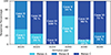 |
Figure 8. Stacked bar chart of relative responses from participants in the second stage of the experiment. Lower segments represent the percentage of responses in which the stimulus with lower atmospheric turbulence was judged more annoying. Upper segments correspond to responses in which the stimulus with higher atmospheric turbulence was judged more annoying. Colors indicate the meteorological conditions A, B, and C as defined in Table 1. Each stimulus pair received 29 ratings. |
Participants showed a clear preference when comparing meteorological conditions A and C, which resulted in the lowest and highest standard deviations of log-amplitude fluctuations, respectively (see Tab. 1). For the A340, meteo condition C was rated more annoying than meteo condition A by 26 out of 29 participants (Chi-squared test, p = 0.0053). Similarly for the A320, meteo condition C was rated as more annoying than meteo condition A by 22 participants, although this result did not reach statistical significance (p = 0.1544).
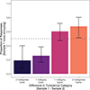 |
Figure 9. Proportion of responses (Choice1) in which Stimulus 1 was judged as more annoying than Stimulus 2 as a function of relative turbulence difference, averaged over all participants and both aircraft types. Error bars indicate 95% CI. |
Comparisons involving meteorological condition B, which produced intermediate standard deviations of log-amplitude fluctuations, showed mixed results. For the A320 aircraft, meteo condition C was unanimously rated as more annoying than condition B (29 participants vs 0). Meteo condition B was rated as more annoying compared to condition A by 19 out of 29 participants (p = 0.7043). For the A340 aircraft, meteo condition C was rated more annoying compared to condition B by 21 out of 29 participants. Meteo condition B was rated as more annoying compared to condition A by only 10 out of 29 participants (p = 0.7043).
The results of comparisons between meteo condition A and meteo condition B indicate little evidence of any reliable perceptual differences between these conditions.
4.3 Mixed-effects analysis of pairwise annoyance judgments
Figure 9 shows the proportion of Choice1 responses (i.e., when Stimulus 1 was judged as more annoying than Stimulus 2), which served as the DV for the regression (Model 1). The influence of turbulence is visualized on the x-axis, showing fewer “more annoying” responses for Stimulus 1 when it was one or two turbulence categories lower than Stimulus 2 (i.e., A–B / B–C; A–C, respectively). This is confirmed by the statistical analysis, which shows increasing odds of a “more annoying” response when turbulence increases (see Tab. 3).
Log-odds (Coef.), Odds Ratios (ORs) with 95% CI for Model 1, predicting the probability of Stimulus 1 being chosen as “more annoying" than Stimulus 2.p-values from Wald z-tests of the null hypothesis that the coefficient equals zero (OR = 1), unadjusted for multiple comparisons.
Controlling for Aircraft type, the odds of being chosen as “more annoying” are approximately 6.7 times higher when the stimulus is one turbulence category higher (Meteo diff. = + 1), and 8.6 times higher when the stimulus is two turbulence categories higher (Meteo diff. = + 2), compared to reference level (Meteo diff. = –2). While the former contrasts were both statistically significant (p ≤ 0.002), the odds did not differ significantly between a Meteo difference of –2 (reference) and –1. This suggests that moving from two categories less turbulence to only one category less is associated with a slight increase (38%) in the odds of being “more annoying”, but this increase is not statistically significant. However, it should be noted that the predictor level Meteo difference −1 encompasses multiple comparisons (i.e., A–B / B–C) and not only a single large turbulence difference (like Meteo diff. =2). As Figure 8 suggests, the perceived difference between weak and intermediate turbulence is likely not the same as the perceived difference between intermediate and high turbulence. Averaging over these asymmetric perceptual steps might lead to a noisy estimate and reduce statistical power for detecting a difference despite a numerically higher odds ratio. Aircraft type was not a statistically significant predictor (p = 0.28, see Tab. 3). A likelihood ratio test comparing models with and without Aircraft type showed no significant improvement in model fit (χ 2[1]=1.17, p = 0.28). This indicates that Aircraft type did not systematically affect annoyance ratings or contribute meaningful explanatory value beyond Meteo difference. Model 2 confirmed the trends in the data: An increase in turbulence category is associated with an increased probability to be chosen as more annoying. According to both models, there was no detectable between-group variance, meaning that participants did not differ systematically in baseline outcome probability after accounting for fixed effects. The fixed effects alone explain approximately 19.4% of the model’s variance (marginal R 2 = 0.194), and the random intercept does not contribute additional explanatory power (conditional R 2 = 0.194; [28]).
5 Discussion
A recently introduced model for turbulence-induced amplitude fluctuations in aircraft flyover sound valid in the unsaturated and partially-saturated scattering regime has been applied to generate realistic aircraft flyover auralizations under varying meteorological conditions. The auralizations were used in listening experiments to investigate the perceptual effects of turbulence-induced fluctuations in aircraft noise under controlled laboratory conditions. In the first stage of the experiments, 12 expert listeners performed two-alternative forced choice (2-AFC) tasks to assess the distinguishability of two different meteorological conditions associated with low and strong amplitude fluctuations respectively. In the second stage, 29 participants, including both expert and naive listeners, rated the relative annoyance of auralized aircraft flyovers in a 2-AFC task. The second stage included three different meteorological conditions, where the additional condition led to intermediate amplitude fluctuations.
5.1 Key results
The results of the first experiment demonstrate that different meteorological conditions lead to significant perceptual differences in the resulting auralizations(p < 0.005), allowing the null hypothesis of chance responses to be rejected. However, the perceptual difference between very low amplitude fluctuations and the baseline auralization without turbulence filtering was too small to be reliably detected, even by expert listeners. Although the difference is audible for the authors, the 20 s sample duration likely contributed to the difficulty in distinguishing subtle amplitude variations even for expert listeners. The meteorological conditions associated with these weak fluctuations can occur in the early morning before sunrise, characterized by shallow stable atmospheric boundary layers that suppress turbulence.
In the second experiment, a clear dependence of relative annoyance on meteorological conditions was observed, aligning with the findings of earlier studies, such as Schaffer et al. [14], which also reported a link between annoyance ratings and random amplitude modulations. Statistical analyses showed stimuli with more turbulence to be associated with a significantly higher odds of being perceived as “more annoying” (ORs ≈ 6–8). While an interaction between Aircraft type and Meteo difference was not found to be statistically significant in the models, there was some apparent interplay between the annoyance caused by turbulence-induced fluctuations and that caused by tonal components, such as engine fan tones. Comments on the questionnaires indicate that participants’ annoyance responses can be broadly categorized into two distinct groups, with some listeners being primarily annoyed by the fluctuating amplitude and others being more disturbed by the high-pitched, whistling fan tones. The two groups can be found for both expert and naive listeners. For example, in the comparison of A320 Meteo A (lowest turbulence category) vs Meteo C (highest turbulence category), 76% of responses indicated that Meteo C was more annoying. In contrast, for the comparison of A320 Meteo B (intermediate turbulence category) vs Meteo C, 100% of responses indicated Meteo C as more annoying. At first sight, this suggests that the increase in relative annoyance is more pronounced when moving from intermediate to strong turbulence than from low to strong turbulence. However, this effect is likely driven by an interaction with fan tones, which are perceived as very annoying in the low turbulence cases, but less so as soon as the effect of atmospheric turbulence becomes more prominent. Specifically, participants noted that fan tones, perceived as particularly piercing in the low turbulence category, became less intrusive in higher turbulence categories. Therefore, in the comparison between intermediate and high turbulence, the fan tones presumably had a much smaller effect on the relative annoyance than in the comparison between low and high turbulence, so that the responses were mainly influenced by the random fluctuations. The presence of strong fan tones could explain why case IV (A340, Meteo A) was rated as more annoying than case V (A340, Meteo B) in 66% of responses. This hypothesis requires further investigation, as the present study was not designed to systematically address the interaction of fan tones and amplitude fluctuations.
The potential importance of fan tones in annoyance ratings has already been addressed by Pieren et al. [18]. They found that the comparison between two aircraft types, of which one exhibits louder audible fan tones compared to the other, showed larger differences in annoyance rating than could be explained by their difference in sound exposure level or the effective perceived noise level.
5.2 Implications for outdoor sound auralization
The findings of this study highlight the importance of accurately modeling turbulence-induced amplitude fluctuations in aircraft flyover auralizations. Firstly, the results confirm that annoyance ratings tend to increase with stronger atmospheric turbulence. Secondly, the data indicate that amplitude fluctuations can interact with other characteristics of aircraft noise such as fan tones and alter the perceptual impact of these characteristics. Therefore, realistic aircraft auralizations should consider accurate models of turbulence-induced amplitude fluctuations as the perceptual impression can be affected in several ways. This effect probably also applies to wind turbines and possibly drones.
So far, earlier aircraft noise annoyance studies using auralized sound stimuli that considered atmospheric turbulence, deliberately chose meteorological conditions that minimize turbulence-induced fluctuations, potentially underestimating their impact [13, 18]. Future research should address the question of which meteorological conditions are suitable for aircraft annoyance studies, and whether multiple conditions must be included to better capture the full spectrum of real-world listening experiences.
5.3 Limitations
The semi-empirical model allows a detailed recreation of the saturation effect for aircraft flyover noise. However, it is more complex to apply to auralizations than the approaches chosen in other current auralization methods [6, 10, 11]. Nevertheless, the semi-empirical model offers greater flexibility in recreating the differences between various meteorological conditions, capturing the seamless transition from the weak-scattering regime to the partially-saturated regime.
The explanatory power of the listening experiment is limited due to the relatively small sample size of 29 participants and the restriction to three different meteorological conditions. Consequently, it is not possible to determine the thresholds above which differences between the conditions can be detected. Furthermore, participants reported difficulty in identifying differences between the samples presented, which were relatively long at 20 s.
Comments from participants and analysis of the results suggest a tendency for individuals to be more annoyed by turbulence-induced amplitude fluctuations, or fan tones. However, this tendency was neither systematically investigated nor reported.
6 Conclusion
In this article, we presented a noise perception study using state-of-the-art aircraft noise auralization tools. We updated these tools to incorporate recent models for turbulence-induced coherence loss and amplitude fluctuations, specifically accounting for the partially-saturated scattering regime.
We were able to show for the first time that atmospheric turbulence can change the annoyance ratings to aircraft noise. Further, the results suggest that amplitude fluctuations can interact with other acoustical characteristics of aircraft noise, like fan tones, and modify their perceptual impact.
Further research is necessary to determine the limits and differences in meteorological conditions, which result in just-audible differences in the resulting auralization. Also, future perceptual studies should address the interaction of turbulence-induced amplitude fluctuations and other aircraft noise characteristics, such as engine fan tones, to better understand the joint impact on aircraft noise annoyance ratings. The authors assume that amplitude fluctuations in aircraft noise lead to aircraft flyovers being perceived more strongly and therefore increase annoyance. Further, flyovers in high turbulence conditions might lead to more night-time awakenings and increased sleep disturbances due to sudden changes in sound pressure level.
In conclusion, since these effects can influence the overall perceptual impression in a number of ways that have not yet been explored, realistic aircraft auralizations should incorporate accurate models of turbulence-induced amplitude fluctuations.
Acknowledgments
The authors would like to thank the participants in the laboratory experiments for their support, and Lothar Bertsch from the German Aerospace Center DLR for providing the aircraft noise emission data. The authors appreciate that SWISSInternational Airlines supplied their flight data recorder data for this study.
Funding
This research was supported by the international research project Localization and Identification Of moving Noise sources (LION) in which the Swiss contribution was funded by the Swiss National Science Foundation (SNSF).
Conflicts of interest
The authors declare that there is no conflict of interest.
Data availability statement
The research data associated with this article are available in Zenodo, under the reference [22].
Supplementary material
Table S1. Log-odds (Coef.), Odds Ratios (ORs) with 95% CI and probabilities (p) for Model 2. Access Supplementary Material
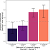 |
FIG. S1. Proportion of responses in which Stimulus 2 was judged as more annoying than Stimulus 1 as a function of relative turbulence difference, averaged over all participants and both aircraft types. Error bars indicate 95% CI. |
References
- J.A. Colosi: Introduction to Acoustic Fluctuations. Cambridge University Press, Cambridge, 2016, pp. 144–184. [Google Scholar]
- V. Ostashev, D. Wilson: Acoustics in Moving Inhomogeneous Media, 2nd edn. CRC Press, Taylor & Francis Group, Boca Raton, 2016. [Google Scholar]
- V.E. Ostashev, D.K. Wilson: Statistical characterization of sound propagation over vertical and slanted paths in a turbulent atmosphere. Acta Acustica united with Acustica 104, 4 (2018) 571–585. [CrossRef] [Google Scholar]
- M.J. Kamrath, V.E. Ostashev, D.K. Wilson, M.J. White, C.R. Hart, A. Finn: Vertical and slanted sound propagation in the near-ground atmosphere: amplitude and phase fluctuations. The Journal of the Acoustical Society of America 149, 3 (2021) 2055–2071. [Google Scholar]
- V.E. Ostashev, M.J. Kamrath, D.K. Wilson, M.J. White, C.R. Hart, A. Finn: Vertical and slanted sound propagation in the near-ground atmosphere: coherence and distributions. The Journal of the Acoustical Society of America 150, 4 (2021) 3109–3126. [Google Scholar]
- A.P.C. Bresciani, J. Maillard, L.D. de Santana: Physics-based scintillations for outdoor sound auralization. The Journal of the Acoustical Society of America 154, 2 (2023) 1179–1190. [CrossRef] [PubMed] [Google Scholar]
- F. Rietdijk, J. Forssén, K. Heutschi: Generating sequences of acoustic scintillations. Acta Acustica united with Acustica 103, 2 (2017) 331–338. [CrossRef] [Google Scholar]
- G. Daigle, J. Piercy, T. Embleton: Effects of atmospheric turbulence on the interference of sound waves near a hard boundary. The Journal of the Acoustical Society of America 64 (1978) 622–630. [Google Scholar]
- A.P.C. Bresciani, J. Maillard, A. Finez: Wind farm noise prediction and auralization. Acta Acustica 8 (2024) 15. [CrossRef] [EDP Sciences] [Google Scholar]
- A. Prescher, A. Moreau, S. Schade: Model for random atmospheric inhomogeneities in engine noise auralization. CEAS Aeronautical Journal 15, 4 (2024) 1111–1125. [Google Scholar]
- J. Forssén: Scintillating and decorrelating signals for different propagation paths in a random medium. Applied Acoustics 221 (2024) 110038. [Google Scholar]
- D. Lincke, R. Pieren: Auralization of atmospheric turbulence-induced amplitude fluctuations in aircraft flyover sound based on a semi-empirical model. Acta Acustica 8 (2024) 18. [Google Scholar]
- R. Pieren, L. Bertsch, D. Lauper, B. Schäffer: Improving future low-noise aircraft technologies using experimental perception-based evaluation of synthetic flyovers. Science of The Total Environment 692 (2019) 68–81. [CrossRef] [Google Scholar]
- B. Schäffer, R. Pieren, S.J. Schlittmeier, M. Brink: Effects of different spectral shapes and amplitude modulation of broadband noise on annoyance reactions in a controlled listening experiment. International Journal of Environmental Research and Public Health 15, 5 (2018) 1029. [CrossRef] [PubMed] [Google Scholar]
- B. Schäffer, S.J. Schlittmeier, R. Pieren, K. Heutschi, M. Brink, R. Graf, J. Hellbrück: Short-term annoyance reactions to stationary and time-varying wind turbine and road traffic noise: a laboratory study. Acoustical Society of America Journal 139 (2016) 2949–2963. [Google Scholar]
- H. Hafke-Dys, T. Kaczmarek, A. Preis, A. Biniakowski, P. Kleka: Noise annoyance caused by amplitude modulated sounds resembling the main characteristics of temporal wind turbine noise. Archives of Acoustics 41, 2 (2016) 221–232. [Google Scholar]
- R. Pieren, D. Lincke: Auralization of aircraft flyovers with turbulence-induced coherence loss in ground effect. The Journal of the Acoustical Society of America 151, 4 (2022) 2453–2460. [CrossRef] [PubMed] [Google Scholar]
- R. Pieren, I. Le Griffon, L. Bertsch, A. Heusser, F. Centracchio, D. Weintraub, C. Lavandier, B. Schäffer: Perception-based noise assessment of a future blended wing body aircraft concept using synthesized flyovers in an acoustic VR environment – The ARTEM study. Aerospace Science and Technology 144 (2024) 108767. [CrossRef] [Google Scholar]
- Z. Sorbjan: Decay of convective turbulence revisited. Boundary-Layer Meteorology 82, 3 (1997) 503–517. [CrossRef] [Google Scholar]
- V.E. Ostashev, D.K. Wilson: Strength and wave parameters for sound propagation in random media. The Journal of the Acoustical Society of America 141, 3 (2017) 2079–2092. [Google Scholar]
- D. Lincke, T. Schumacher, R. Pieren, Synthesizing coherence loss by atmospheric turbulence in virtual microphone array signals. The Journal of the Acoustical Society of America 153, 1 (2023) 456–466. [CrossRef] [PubMed] [Google Scholar]
- D. Lincke, R. Pieren: Aircraft auralizations with turbulence-induced amplitude fluctuations for listening experiment. https://doi.org/10.5281/zenodo.15352261 (2025). [Google Scholar]
- P. Virtanen, R. Gommers, T.E. Oliphant, M. Haberland, T. Reddy, D. Cournapeau, E. Burovski, P. Peterson, W. Weckesser, J. Bright, S.J. van der Walt, M. Brett, J. Wilson, K.J. Millman, N. Mayorov, A.R.J. Nelson, E. Jones, R. Kern, E. Larson, C.J. Carey, İ. Polat, Y. Feng, E.W. Moore, J. VanderPlas, D. Laxalde, J. Perktold, R. Cimrman, I. Henriksen, E.A. Quintero, C.R. Harris, A.M. Archibald, A.H. Ribeiro, F. Pedregosa, P. van Mulbregt: SciPy 1.0 Contributors. SciPy 1.0: fundamental algorithms for scientific computing in python. Nature Methods 17 (2020) 261–272. [CrossRef] [Google Scholar]
- Y. Benjamini, Y. Hochberg: Controlling the false discovery rate: a practical and powerful approach to multiple testing. Journal of the Royal Statistical Society. Series B (Methodological) 57, 1 (1995) 289–300. [Google Scholar]
- R Core Team: R: A Language and Environment for Statistical Computing. R Foundation for Statistical Computing, Vienna, Austria, 2021. [Google Scholar]
- M.E. Brooks, K. Kristensen, K.J. van Benthem, A. Magnusson, C.W. Berg, A. Nielsen, H.J. Skaug, M. Maechler, B.M. Bolker: glmmTMB balances speed and flexibility among packages for zero-inflated generalized linear mixed modeling. The R Journal 9, 2 (2017) 378–400. [Google Scholar]
- M. McGillycuddy, D.I. Warton, G. Popovic, B.M. Bolker: Parsimoniously fitting large multivariate random effects in glmmTMB. Journal of Statistical Software 112, 1 (2025) 1–19. [Google Scholar]
- S. Nakagawa, P.C.D. Johnson, H. Schielzeth: The coefficient of determination R2 and intra-class correlationcoefficient from generalized linear mixed-effects models revisited and expanded. Journal of The Royal Society Interface 14, 134 (2017) 20170213. [Google Scholar]
Cite this article as: Lincke D. Kawai C. & Pieren R. 2025. Atmospheric turbulence affects noise annoyance from aircraft yovers. Acta Acustica, 9, 69. https://doi.org/10.1051/aacus/2025053.
All Tables
Overview of considered cases and limit frequency f lim (Hz) indicating the theoretical boundary between weak-scattering and strong-scattering regime for the moment of direct flyover.
Log-odds (Coef.), Odds Ratios (ORs) with 95% CI for Model 1, predicting the probability of Stimulus 1 being chosen as “more annoying" than Stimulus 2.p-values from Wald z-tests of the null hypothesis that the coefficient equals zero (OR = 1), unadjusted for multiple comparisons.
All Figures
|
Figure 1. Geometry of aircraft flyover. |
| In the text | |
|
Figure 2. Frequency dependency of log-amplitude fluctuation |
| In the text | |
|
Figure 3. Statistical magnitude responses of amplitude modulation (AM) filters to reproduce turbulence-induced amplitude fluctuations for different cases. The curves show the upper and lower bounds of the 68% confidence bands at shortest distance of the aircraft. |
| In the text | |
|
Figure 4. Modulation spectrum of level fluctuations in octave bands. Black curve indicated mean fluctuation of measurements presented in [12]. Error bars indicate standard deviation of measurements. Orange line represents modulation spectrum of synthesized fluctuations. |
| In the text | |
|
Figure 5. Generated level fluctuations for case I in the 2 kHz octave band. The standard deviation of this signal is 2.6 dB. |
| In the text | |
|
Figure 6. Spectrograms of auralized Airbus A320 in low and high turbulence conditions. Top: low turbulence condition A (case I); Bottom: high turbulence condition C (case III). |
| In the text | |
|
Figure 7. Spectrograms of auralized Airbus A340 in low and high meteorological turbulence conditions. Top: low turbulence condition A (case IV); Bottom: high turbulence condition C (case VI). |
| In the text | |
|
Figure 8. Stacked bar chart of relative responses from participants in the second stage of the experiment. Lower segments represent the percentage of responses in which the stimulus with lower atmospheric turbulence was judged more annoying. Upper segments correspond to responses in which the stimulus with higher atmospheric turbulence was judged more annoying. Colors indicate the meteorological conditions A, B, and C as defined in Table 1. Each stimulus pair received 29 ratings. |
| In the text | |
|
Figure 9. Proportion of responses (Choice1) in which Stimulus 1 was judged as more annoying than Stimulus 2 as a function of relative turbulence difference, averaged over all participants and both aircraft types. Error bars indicate 95% CI. |
| In the text | |
|
FIG. S1. Proportion of responses in which Stimulus 2 was judged as more annoying than Stimulus 1 as a function of relative turbulence difference, averaged over all participants and both aircraft types. Error bars indicate 95% CI. |
| In the text | |
Current usage metrics show cumulative count of Article Views (full-text article views including HTML views, PDF and ePub downloads, according to the available data) and Abstracts Views on Vision4Press platform.
Data correspond to usage on the plateform after 2015. The current usage metrics is available 48-96 hours after online publication and is updated daily on week days.
Initial download of the metrics may take a while.