| Issue |
Acta Acust.
Volume 9, 2025
|
|
|---|---|---|
| Article Number | 68 | |
| Number of page(s) | 15 | |
| Section | Musical Acoustics | |
| DOI | https://doi.org/10.1051/aacus/2025049 | |
| Published online | 31 October 2025 | |
Scientific Article
Nonlinear acoustics in brass instruments using 2D complex modal bases
1
Aix Marseille Univ, CNRS, Centrale Med, LMA UMR7081, 4 impasse Nikola Tesla, 13013 Marseille, France
2
Yamaha Corporation, Research and Development Division, 10-1, Nakazawa-cho, Chuo-ku, Hamamatsu-shi, Shizuoka, 430-8650, Japan
* Corresponding author: This email address is being protected from spambots. You need JavaScript enabled to view it.
Received:
16
June
2025
Accepted:
8
September
2025
Abstract
The modelling approach presented here aims at developing accurate, yet computationally efficient, numerical models of brass instrument resonators including nonlinear propagation, viscothermal losses and radiation effects in 2D axisymmetric domains. The central idea is to bridge the refined accuracy of 2D models with the efficiency of reduced-order modal approaches. To model the nonlinear acoustic propagation inside the resonator, we propose the use of the Blackstock equation, a more appropriate choice when dealing with nonlinear standing wave motion, compared to the more commonly used Burgers equation. The first step of the approach consists in obtaining a complex modal basis from a 2D axisymmetric finite element model of the linearized equations. Here, a bounded domain outside the resonator, with a nonreflecting boundary condition, is included to explicitly account for 2D radiation effects. Moreover, the effects of the viscothermal boundary layers at the interior walls are modelled efficiently through an impedance boundary condition. The Blackstock equation is then projected onto the resulting 2D complex modal basis, leading to a compact set of nonlinear ordinary differential equations (ODEs) that can be truncated at any suitable number of terms. This leads to exploitable reduced formulations, adapted to quick temporal simulations, bifurcation analysis or parametric studies, retaining nevertheless the accuracy provided by 2D axisymmetric models. Additionally, the explicit account of the exterior acoustic field allows for the calculation of radiated sound pressures as well as directivity patterns, contrary to typical 1D models. Experimental validation and illustrative numerical results are presented for a simplified trumpet geometry in both linear and nonlinear scenarios, highlighting the benefits of the proposed approach.
Key words: Nonlinear acoustic propagation / Brass instruments / Complex modes / 2D axisymmetric model / Reduced-order models
© The Author(s), Published by EDP Sciences, 2025
 This is an Open Access article distributed under the terms of the Creative Commons Attribution License (https://creativecommons.org/licenses/by/4.0), which permits unrestricted use, distribution, and reproduction in any medium, provided the original work is properly cited.
1 Introduction
The physical modeling of brass wind instruments has received considerable attention in the last few decades [1]. These instruments constitute complex physical systems that, from the point of view of physical modeling, still present many challenging aspects. These include the nonlinear interaction between the lip vibration and the acoustics of the resonator [2], nonlinear acoustic propagation inside the bore [3], viscothermal losses occurring at the inner walls [4], radiation directivity, among others. In this work, our focus is on the modelling of the instrument itself, i.e., without the influence of the lip vibration and the associated control by the musician.
Previous studies have, by and large, employed relatively simple models to study the acoustics of brass horns. Typically framed in one-dimensional contexts, most developed models were aimed at reproducing the fundamental features of these instruments. One generally seeks simplified models for their physical interpretability and low-computational cost, which allow for more in-depth analysis as well as computationally intensive tasks like parametric studies, optimization or sound synthesis. However, despite their general ability to reproduce behavior observed experimentally, at least qualitatively, simplified models often present inherent limitations that prevent them from capturing the more subtle features of real instruments. For example, 1D models often rely on the assumption of plane wave propagation which, albeit reasonable in the narrower parts of the instrument, clearly breaks down at the exit of the instrument. Even though spherical wave propagation models have already been proposed to treat this issue [5], these are not guaranteed to reproduce the complex nature of pressure fields at these junctures. Moreover, the radiative boundary conditions need to be enforced at the exit of the instrument, often based on approximate models [6], representing another important source of error. Finally, 1D models typically aim to reproduce acoustic fields solely inside the instrument, providing little information about the radiated sound which is, ultimately, one of the most important criteria to assess the instruments’ quality.
Another important aspect is related to nonlinear acoustic propagation inside the resonator, particularly a relevant feature influencing the timbre of brass instruments [7]. Although many studies have dealt with this topic, modeling efforts almost exclusively rely on the Burgers’ equation [8, 9]. However, this equation assumes only forward or backward propagating waves and its use in the context of brass instruments is (at least) questionable, since standing waves are formed inside the instrument.
In the commercial contexts, for example, where manufacturers are interested in optimizing/fine-tuning certain aspects of their instruments, the accuracy provided by these models often falls short of the desired goals. Therefore, there is a need for more refined models, that can reliably capture the finer details missed by simplified ones. On the other hand, refined higher-order models can (and have) been pursued, in both 2D or 3D numerical domains and using different models for the acoustics [10, 11]. Needless to say that, in general, these models entail large computational costs and, although able to provide refined physical descriptions at specific configurations, are inadequate for parametric studies, optimization, bifurcation analysis, etc.
The motivation behind this work lies on the need to build a physical model that provides: (1) an accurate description of the pertinent acoustic phenomena, including nonlinear propagation, viscothermal losses as well as 2D propagation and radiation effects, and also (2) an efficient/exploitable framework (low computational cost) that can be used for relatively quick temporal simulations, parametric studies, optimization, bifurcation analysis, etc. The approach proposed here aims to bridge the accuracy provided by 2D-axisymmetric models and the efficiency of reduced-order modal approaches. The general idea consists in using a 2D finite element (FE) model of the linearized equations to obtain a suitable modal basis that can then be used to project the nonlinear acoustics equation, leading to exploitable reduced-order models (composed of a truncated set of nonlinear ordinary differential equations (ODEs)). An illustrative diagram of the proposed approach is shown in Figure 1 (Note: symbols appearing in Figure 1 will be defined in the following sections).
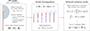 |
Figure 1 Illustrative scheme of the proposed modeling approach: (1) discretize 2D linear problem via FE model; (2) compute the complex modal basis from the associated quadratic eigenvalue problem; (3) projection of nonlinear acoustics PDE onto complex modal basis. |
By considering an exterior acoustic field (outside the flaring horn), the 2D FE model allows us to explicitly model the radiated sound field, bypassing issues related to the choice of a suitable propagation and/or radiation impedance model (plane or spherical waves [5]) unavoidable when using typical one-dimensional models. Additionally, the viscothermal losses at the walls represent a linear phenomenon (albeit with an intricate frequency dependency [4]) and can hence be included in the FE model. The latter will be modeled via an impedance boundary condition, an efficient approach that avoids solving explicitly the (usually very thin) acoustic boundary layers [12].
Due to the localized nature of the modeled energy dissipation mechanisms (viscothermal and radiation losses), the eigenvalue problem stemming from the 2D FE model leads to a complex modal basis [13]. Contrary to real normal modes, complex modes contain phase information that essentially encapsulate the localized (or unevenly distributed) nature of the dissipation mechanisms.
In this particular context, the full potential of modal decomposition is highlighted. Firstly, the modal basis serves to spatially discretize the problem. Secondly, because modes have characteristic natural frequencies, they can also serve to discretize the system in the frequency domain, i.e., modes whose natural frequencies fall outside the frequency bands of interest can generally be neglected. Notably, this property is useful for mitigating numerical dispersion, a common problem when solving wave equations using finite difference or finite elements methods in the time domain [14]. Thirdly, modes have characteristic damping ratios which represent, in a simple manner, the often-times intricate dissipation mechanisms. For example, viscothermal losses are notably difficult to model in the time-domain since they give rise to fractional-order derivatives [15]. These can however be easily represented in a modal framework, suited for both frequency and time-domain analysis. Finally, modal approaches are able to represent nonlinear terms via constant tensors which, although generally dense (inducing modal coupling), have been proven useful to treat nonlinear problems in an efficient manner [16, 17].
In Section 2, the derivation of the nonlinear acoustics model is presented. Section 3 describes the 2D FE discretization, computation of complex modes, and the subsequent formulation of the reduced-order model. Section 4 presents illustrative numerical results on a simplified trumpet geometry, used here as a study case. Finally, experimental validation, in both linear and nonlinear scenarios, is presented in Section 5.
2 Model description
2.1 Nonlinear acoustics in 3D domains
In most applications, not involving explosions or other supersonic events, nonlinear acoustics are typically modeled through what are often called weakly-nonlinear models. Starting from the set of irrotational compressible Euler equations and a state equation for the fluid, a wide variety of models have been proposed over the years, well documented in an historical review by Jordan [18]. Of particular interest to us, are the so-called wave equations, where the acoustic field is represented by a single scalar variable. When deriving wave-like formulations in the context of weakly-nonlinear acoustics models, one of the first results appears as the Söderholm equation [18, 19], written here in its lossless form, in terms of the velocity potential ϕ([ B O L D ]x, t)
 (1)
(1)
where the over-dot denotes temporal derivatives, ∇ and Δ are the gradient and Laplacian operators, c is the speed of sound in the fluid, and γ its adiabatic index. Note that the acoustic pressure and velocity can be easily obtained from the derivatives of the velocity potential via  and [
B
O
L
D
]v([
B
O
L
D
]x, t)=∇ϕ. In equation (1) we can easily identify the linear wave equation and three nonlinear terms, two quadratic and one cubic. Lower-order approximations can be derived, valid in more constricted amplitude ranges. For example, neglecting the cubic term in equation (1) leads to the second-order approximation known as the Blackstock equation [20]
and [
B
O
L
D
]v([
B
O
L
D
]x, t)=∇ϕ. In equation (1) we can easily identify the linear wave equation and three nonlinear terms, two quadratic and one cubic. Lower-order approximations can be derived, valid in more constricted amplitude ranges. For example, neglecting the cubic term in equation (1) leads to the second-order approximation known as the Blackstock equation [20]
 (2)
(2)
By the substitution corollary [21], we can replace the first order approximation  in the last nonlinear term
  such that it is transformed into
  leading to the lossless form of the famous Kuznetsov equation
 (3)
(3)
The lossless forms of the Blackstock (2) and Kuznetsov (3) equations are both second-order approximations and represent equivalent physical models [22]. However, the Kuznetsov equation presents a nonlinear term involving a second-order time derivative  that can lead to numerical difficulties, for example, when performing temporal integration using explicit schemes. In these contexts, the Blackstock formulation is a more appropriate choice. Furthermore, we will see later that the nonlinear terms in the Blackstock equation lead to more compact formulations when using modal approaches. As a side note, the lossless forms of the popular Westervelt and Burgers’ equations can be derived directly from the second-order approximations shown here. Neglecting the first nonlinear term in equation (3) leads to the Westervelt equation and further assuming strictly forward propagating waves, in a 1D context, leads to the inviscid Burgers’ equation [23].
All these models represent the cumulative nature of nonlinear acoustic propagation and are hence able to reproduce wave-steepening phenomena and the development of shock waves. However, their ability to describe these phenomena accurately differs quantitatively. The ranges of validity for nonlinear wave equations are typically given in terms of the acoustic Mach number M = u/c. For the third-order Söderholm equation, a rough estimate is given in [24] as M < 0.7, while it is approximately M < 0.1 for the second-order Blackstock/Kuznetsov equations. In this work, we opted for the Blackstock equation as a good compromise between model complexity and accuracy. It is likely that this model is plausible for moderate-to-high dynamic levels in real playing conditions. However, neglecting higher-order terms could eventually induce errors at extreme dynamics levels, particularly near the formation of shock waves. Nevertheless, the formulation presented here can be extended to higher-order models with relative ease.
2.2 Nonlinear formulation for 3D-axisymmetric problems in cylindrical coordinates
Brass instruments are made up of long pipes with variable cross-section along their central axis. In most cases, pipes are bent at several locations to render them more compact. Some studies have underlined that curved duct bents can induce some mistuning and/or added dissipation in the response of brass instruments [25]. However, for sufficiently smooth bents in relatively narrow ducts, these effects can be considered negligible in a first approximation. Under this assumption, we can consider the instrument as an axisymmetric object and the equations derived previously can be significantly simplified, i.e., we can transform the generic 3D model (2) into an axisymmetric 2D formulation in cylindrical coordinates (r, z, φ), where r, z and φ are the radial, longitudinal and angular coordinates, respectively.
The Blackstock equation (2) in cylindrical coordinates can be written as
![Mathematical equation: $$ \begin{aligned}&\ddot{\phi }-c^{2} \left[\frac{1}{r} \frac{\partial }{\partial r} \left(r\frac{\partial \phi }{\partial r} \right)+\frac{1}{r^{2} } \frac{\partial ^{2} \phi }{\partial \varphi ^{2} } +\frac{\partial ^{2} \phi }{\partial z^{2} } \right] \nonumber \\&+2\left(\frac{\partial \dot{\phi }}{\partial r} +\frac{1}{r} \frac{\partial \dot{\phi }}{\partial \varphi } +\frac{\partial \dot{\phi }}{\partial z} \right)\left(\frac{\partial \phi }{\partial r} +\frac{1}{r} \frac{\partial \phi }{\partial \varphi } +\frac{\partial \phi }{\partial z} \right) \nonumber \\&+(\gamma -1)\dot{\phi }\left[\frac{1}{r} \frac{\partial }{\partial r} \left(r\frac{\partial \phi }{\partial r} \right)+\frac{1}{r^{2} } \frac{\partial ^{2} \phi }{\partial \varphi ^{2} } +\frac{\partial ^{2} \phi }{\partial z^{2} } \right]=0. \end{aligned} $$](/articles/aacus/full_html/2025/01/aacus250077/aacus250077-eq9.gif) (4)
(4)
Furthermore, because we consider an axisymmetric domain, the derivatives with respect to the azimuthal angle,  vanish, and hence equation (4) simplifies to
![Mathematical equation: $$ \begin{aligned}&\ddot{\phi }-c^{2} \left[\frac{1}{r} \frac{\partial }{\partial r} \left(r\frac{\partial \phi }{\partial r} \right)+\frac{\partial ^{2} \phi }{\partial z^{2} } \right] \nonumber \\&+2\left(\frac{\partial \dot{\phi }}{\partial r} +\frac{\partial \dot{\phi }}{\partial z} \right)\left(\frac{\partial \phi }{\partial r} +\frac{\partial \phi }{\partial z} \right) \nonumber \\&+ (\gamma -1)\, \dot{\phi }\left[\frac{1}{r} \frac{\partial }{\partial r} \left(r\frac{\partial \phi }{\partial r} \right)+\frac{\partial ^{2} \phi }{\partial z^{2} } \right]=0. \end{aligned} $$](/articles/aacus/full_html/2025/01/aacus250077/aacus250077-eq11.gif) (5)
(5)
At this point it must be highlighted that total length L of a brass instrument is generally much larger than its characteristic radial dimensions S(z). Consequently, acoustic perturbations inside the instrument’s bore are composed essentially of plane waves. This assumption breaks down only near the exit of the instrument, where the cross-section is larger. Because of the larger cross-section, acoustic levels near the exit of the instrument are also relatively weaker. With that said, large amplitude acoustic perturbations and hence nonlinear propagation are known to develop primarily at the narrower parts of the horn, where the plane wave assumption is reasonable. This leads us to the conclusions that, in the context of brass instruments, the nonlinear terms in equation (5) involving the radial derivative  can confidently be neglected. Finally, equation (5) can be simplified to
![Mathematical equation: $$ \begin{aligned}&\ddot{\phi }-c^{2} \left[\frac{1}{r} \frac{\partial }{\partial r} \left(r\frac{\partial \phi }{\partial r} \right)+\frac{\partial ^{2} \phi }{\partial z^{2} } \right] \nonumber \\&+2\left(\frac{\partial \dot{\phi }}{\partial z} \right)\left(\frac{\partial \phi }{\partial z} \right) \nonumber \\&+(\gamma -1)\dot{\phi }\left(\frac{\partial ^{2} \phi }{\partial z^{2} } \right)=0 \end{aligned} $$](/articles/aacus/full_html/2025/01/aacus250077/aacus250077-eq13.gif) (6)
(6)
a 2-D formulation where only two quadratic nonlinear terms subsist.
2.3 Free-field radiation and non-reflecting boundary condition
In commonly used one-dimensional acoustic models, one has to consider which type of radiating boundary condition to impose at the open-end of a flaring horn. A wide variety of approximate models can be used, with different degrees of accuracy, considering either plane or spherical wave propagation [5, 6]. Moreover, one-dimensional models are geared towards a description of the acoustic field inside the resonator but provide little information about the radiated sound field, which can be useful to calculate radiation efficiency parameters or directivity patterns. In two-dimensional models these questions are not posed since the pressure fields outside the open-end can be calculated explicitly, when considering an exterior field. Hence, two-dimensional models are not only more accurate, but can also provide extra information regarding the radiative character of the studied instrument.
The typical framework for this type of 2D models involves the consideration of an exterior domain with special boundary conditions, aimed at simulating an anechoic environment, as illustrated in Figure 2 (boundary Γr). Here, one needs to treat that fact that an unbounded (infinite) domain is to be modeled by a necessarily bounded (finite) computational domain. For exterior acoustics problems, solutions must obey the Sommerfeld radiation condition at infinity [26]
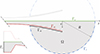 |
Figure 2 Diagram of the considered axisymmetric model. The dashed and dash-dotted lines correspond to the viscothermal Γ v t and radiative Γ r boundaries, respectively. |
 (7)
(7)
where k is the wavenumber and ξ = ∥[ B O L D ]x∥ is a radius centered near the origin of the sound source. It essentially states that, sufficiently far away from the source, solutions allow only outgoing waves. Methods to approximate this condition numerically typically involve either infinite elements, thin absorbing layers (perfectly matched layers) or non-reflecting boundary conditions, as described extensively in the reviews [27] or [28]. These attempt to minimize spurious reflections (incoming waves) in the artificially bounded domain (here a sphere of radius R). Depending on the nature of the exterior problem and the type of radiating sources involved, different methods can be more or less appropriate, and chosen based on criteria of accuracy and/or computational efficiency. Here we have used one of the simplest and most widely used non-reflecting boundary condition, where a relation between the unknown solution and its radial (normal) derivative is imposed at the boundary of the spherical enclosure Γ r . It was first proposed by Bayliss and Turkel [29] and is written in the frequency domain as
 (8)
(8)
It represents a first-order approximation of equation (7) that is easy to implement in FE models and effective in simple scenarios like ours, i.e. a relatively well-defined location of the radiating “source" (horn’s open-end) centered around a spherical domain. The choice of the radius R of the spherical exterior domain will always be a compromise between accuracy and computational time. That is, a larger R will better approximate the limiting Sommerfeld condition (7) but will also lead to larger systems and hence larger computational cost. In this work, values of about 0.15 < R/L < 0.5 were typically used. From our experience, relatively small exterior fields (say R ≈ L/6) do not affect significantly the predicted modal frequencies nor damping ratios. However, when calculating far-field directivity patterns for example, a larger R is typically well-advised, for improved accuracy (particularly for lower-order modes where wavelengths are large) but also to mitigate potential near-field effects.
2.4 Viscothermal losses modeled by an impedance boundary condition
Aside from the radiation losses discussed above, another important energy dissipation mechanism is musical resonators are the viscothermal losses related to the nature of the acoustic field near the interior walls [30]. In light fluids, bulk (or compressible) viscous effects are very small and generally neglected, even though these can eventually play a role in the presence of shock waves [31]. Near the wall interface, acoustic perturbations will form “acoustic boundary layers" within which acoustic variables change drastically. In these layers, the shear motion enforced by the no-slip boundary condition will generate viscous and thermal dissipative effects. These can be modeled explicitly using the linearized, compressible Navier-Stokes equations, albeit at a high computational cost. Not only do extra field variables must be accounted for (velocity, temperature, etc.), but also the often very thin boundary layers need to be discretized. Hence, many efforts have been made over the years to find efficient ways to approximate these dissipative effects [4].
These phenomena are notably difficult to model in the time domain, since fractional-order derivatives appear in the formulation [9, 15]. This occurs because the boundary layer thicknesses, both thermal δ
t
and viscous δ
v
, are known to be proportional to  . For linear perturbations along a wall’s surface, they are given explicitly by [4]
 (9)
(9)
where ρ is the static density, ν is the kinematic viscosity, κ is the thermal conductivity and C p is the coefficient of specific heat at constant pressure. In the frequency domain however, these problems are not posed. For example, one-dimensional models in the frequency domain (e.g., TMM method), commonly consider complex wavenumbers, which provide reasonable approximations when the waveguide geometry is made up of simple geometric elements (e.g., cylinders, cones) [32].
Nevertheless, in the context of musical instruments, the size of the boundary layers is generally extremely small compared to the characteristic dimensions/wavelengths. In these scenarios, it is enticing to model the phenomena using artificial boundary conditions that mimic the effects of the (thin) boundary layers, while retaining the conservative Helmholtz equation for the acoustic domain. Here, we have followed the model proposed by Berggren et al. [12], that gives the following impedance boundary condition in the frequency domain
 (10)
(10)
Such approaches have proven to be a powerful tool to model wall losses, since they provide accurate approximate solutions at low computational cost and are valid for a wide range of geometries (the only constraint is that the minimum radius of curvature of the considered surface must be larger than the boundary layer – which is largely the case in musical instruments).
3 FE model and complex modal superposition
3.1 FE model
As mentioned before, our aim here is to use a finite element discretization of the linearized system in order to obtain a suitable modal basis, which will serve as a basis of functions on which to subsequently project the nonlinear Blackstock equation. To solve the linearized problem, we assume damped harmonic solutions with angular frequency ω and exponential decay coefficient α. Its temporal character is e λ t , where λ ∈ ℂ is the eigenvalue parameter, expanded as λ = α + i ω. A complex angular wavenumber can then be defined as k = −i λ = ω − i α. Then, the linear axisymmetric problem to be solved in the frequency domain is written in terms of the wavenumber k as
![Mathematical equation: $$ \begin{aligned} {k^{2} \phi -\left[\frac{1}{r} \frac{\partial }{\partial r} \left(r\frac{\partial \phi }{\partial r} \right)+\frac{\partial ^{2} \phi }{\partial z^{2} } \right]=0}&{\, \, \, \, \, \mathrm{in}\, \, \, \Omega } \\ {\left(\frac{1}{R} -ik\right)\phi +\frac{\partial \phi }{\partial n}=0}&{\quad \mathrm{on}~\mathrm \Gamma _{r} } \\ {-\delta _{v} \frac{i-1}{2} \mathrm{\Delta } \phi +\delta _{t} k^{2} \frac{(i-1)(\gamma -1)}{2} \phi +\frac{\partial \phi }{\partial n}=0}&{\quad \mathrm{on}~\mathrm \Gamma _{vt} } \\ {\frac{\partial \phi }{\partial n}=0}&{\quad \mathrm{on}~\mathrm \Gamma _{w,s,e} } \end{aligned} $$](/articles/aacus/full_html/2025/01/aacus250077/aacus250077-eq19.gif) (11)
(11)
where, aside from the boundary conditions already discussed, we include a Neumann boundary condition at Γ w , Γ s and Γ e , corresponding to the exterior walls of the horn (Γ w ), the axis of symmetry (Γ s ) and the boundary at the mouthpiece entry (Γ e ), respectively (see Fig. 2). It is worth noting that the problem is here formulated in term of the acoustic velocity potential ϕ(r, z), but an equivalent formulation for the acoustic pressure can be obtained by replacing directly ϕ(r, z) by p(r, z). This is possible because, in linearized conditions, the pressure and velocity potential are related simply by p(r, z)= − i ω ρ ϕ(r, z) and, because there are no constant (zero-order) terms in the formulation, the factor i ω ρ cancels out upon substitution.
For compactness, here we do not derive the weak formulation or FE discretization procedures involved, as these can be found in reference literature (e.g., [33]). For now, we simply state that second-order (6-node) triangular elements were used and the longest edge of each element h max was kept smaller than one-fifth of the smallest considered wavelength, i.e. h max ≤ 2π/5k max, a commonly used rule-of-thumb. Aside from this upper limit, we have also used refined meshes in narrow regions, notably near the mouthpiece, with at least two elements in the radial direction. All meshes were computed using Comsol Multiphysics. Additionally, we note in passing that FE formulations including nonlinear propagation (Kuznetsov equation) have also been derived recently [34].
3.2 Complex modal decomposition
After the FE discretization of the linear, frequency-domain system (11)–(14), we eventually reach an eigenvalue problem of the form
 (12)
(12)
with complex eigensolutions (λ n , [ B O L D ]w n )∈ℂ. Here, the damping matrix is composed of two sub-matrices [ B O L D ]C(λ)=[ B O L D ]C r + [ B O L D ]C v t (λ) corresponding to the radiation and viscothermal losses, respectively. Notably, the matrix is frequency-dependent and hence we have a nonlinear eigenvalue problem whose matrices depend on the eigenvalues themselves. This class of problems can typically be framed in the context of nonviscous damping models [35], where the modelled dissipative phenomena is non-local in time. That is, they contain “hereditary/memory" effects that cannot be modeled as proportional to the instantaneous velocity (viscous damping).
Despite their particular structure, solving eigenvalue problems of this type (15) poses no significant difficulty. Typically, they need to be solved in an iterative manner [36]. That is, evaluating the frequency-dependent matrices at an initial value λ
0 and solving for (λ
n
, [
B
O
L
D
]w
n
) iteratively, until converged solutions are obtained. Furthermore, in the context of brass instruments, we know that the viscothermal losses will have a small effect on the natural frequencies. Hence, here we solve the problem with a single iteration. In a first step, we solve for N modes ( ,
,  ) of the system without viscothermal losses, i.e. setting [
B
O
L
D
]C
v
t
(λ)=0. Subsequently, we solve for each mode n including the viscothermal losses using
) of the system without viscothermal losses, i.e. setting [
B
O
L
D
]C
v
t
(λ)=0. Subsequently, we solve for each mode n including the viscothermal losses using  . This procedure is generally sufficient for systems where the damping law depends slowing on frequency, as noted by Woodhouse [37] (see p. 556). Some numerical tests have been performed indicating that, for our system, relative errors on the obtained eigenvalues λ
n
are in the order of 10−4% after a single iteration. Naturally, since matrices [
B
O
L
D
]M, [
B
O
L
D
]C and [
B
O
L
D
]K are large (in our case between 500 and 20,000 degrees-of-freedom), the eigenvalue problem must be solved using dedicated solvers [38] that extract only a finite set of N eigensolutions at low computational cost, instead of redundantly solving for the full set of eigensolutions. Here we have used either Matlab’s eigs or Comsol’s inbuilt ARPACK solver (with the latter often being quicker to compute).
. This procedure is generally sufficient for systems where the damping law depends slowing on frequency, as noted by Woodhouse [37] (see p. 556). Some numerical tests have been performed indicating that, for our system, relative errors on the obtained eigenvalues λ
n
are in the order of 10−4% after a single iteration. Naturally, since matrices [
B
O
L
D
]M, [
B
O
L
D
]C and [
B
O
L
D
]K are large (in our case between 500 and 20,000 degrees-of-freedom), the eigenvalue problem must be solved using dedicated solvers [38] that extract only a finite set of N eigensolutions at low computational cost, instead of redundantly solving for the full set of eigensolutions. Here we have used either Matlab’s eigs or Comsol’s inbuilt ARPACK solver (with the latter often being quicker to compute).
In viscously damped systems, decoupling is generally achieved using either real or complex modes, depending on the nature of the damping, classical or non-classical [39], respectively. In nonviscously damped systems, decoupling can also be achieved, even if (bi)orthogonality conditions become slightly more complicated [40]. Here however, we build our model in the more familiar framework of complex modes, assuming a “mode-by-mode" viscous damping. This type of simplification, widely used in musical acoustics [41], is often physically justifiable under certain conditions, eventually even through quantifiable measures [42]. They essentially involve neglecting potential cross-coupling terms stemming from the projection of the frequency-dependent damping matrices onto a complex (viscously damped) modal basis. In our particular case, the (non-local) damping effects are accounted for in-resonance (since each mode n is calculated correctly, i.e., using [
B
O
L
D
]C
v
t
(λ
n
)), but not necessarily off-resonance. However, since we have lightly damped modes with well-separated modal frequencies and, most importantly, a damping law with a slow-varying frequency dependence  , the associated approximation errors are of secondary importance, i.e. the resulting modal matrices are diagonal dominant. With that said, we feel these points are rarely discussed in the musical acoustics literature and are deserving of more attention.
Since [
B
O
L
D
]M, [
B
O
L
D
]C, and [
B
O
L
D
]K are symmetric, eigensolutions occur in pairs of complex conjugates, with eigenvectors  and eigenvalues
 (13)
(13)
where the overbar denotes complex conjugation, ω
n
are the undamped angular frequencies and ζ
n
the modal damping ratios. Once a suitable complex modal basis is obtained, the acoustic field can be expanded in terms of a truncated set of N complex modal pairs. Letting ϕ(t) be the velocity potential evaluated at the nodes of the FE discretized field, we define  and the complex modal transformation is performed in state-space [13], given by
![Mathematical equation: $$ \begin{aligned} \left\{ \begin{array}{c}{\boldsymbol{{\phi }}(t)} \\ {\boldsymbol{ \alpha }(t)}\end{array} \right\}&= {\sum _{n=1}^N}[\boldsymbol{\mathrm{u} }_{n} q_{n} (t)+\bar{\boldsymbol{\mathrm{u} }}_{n} \bar{q}_{n} (t)]\\ \nonumber&={\boldsymbol{\mathrm{Uq} }(t)}+ \bar{\boldsymbol{\mathrm{U} }}\bar{\boldsymbol{\mathrm{q} }}(t)=2\text{ Re}[{\boldsymbol{\mathrm{Uq} }(t)}] \end{aligned} $$](/articles/aacus/full_html/2025/01/aacus250077/aacus250077-eq28.gif) (14)
(14)
where [ B O L D ]q(t) are the modal coordinates, [ B O L D ]u n = [[ B O L D ]w n λ n [ B O L D ]w n ] T are the “extended" modes shapes stemming from the state-space reformulation of system (15)
![Mathematical equation: $$ \begin{aligned} \Bigg (\lambda _n \left[\begin{array}{cc} {\boldsymbol{\mathrm{C} }(\lambda _n)}&{\boldsymbol{\mathrm{M} }} \\ {\boldsymbol{\mathrm{M} }}&{0} \end{array}\right] + \left[\begin{array}{cc} {\boldsymbol{\mathrm{K} }}&{\boldsymbol{\mathrm{0} }} \\ {\boldsymbol{\mathrm{0} }}&-\boldsymbol{\mathrm{M} } \end{array}\right] \Bigg ) \boldsymbol{\mathrm{u} }_n = 0 \end{aligned} $$](/articles/aacus/full_html/2025/01/aacus250077/aacus250077-eq29.gif) (15)
(15)
and the modal matrix [ B O L D ]U is then
![Mathematical equation: $$ \begin{aligned} {\boldsymbol{\mathrm{U} }}=\left[\begin{array}{cc} {\boldsymbol{\mathrm{W} }} \\ {\boldsymbol{\mathrm{W} }\boldsymbol\mathrm{\Lambda }} \end{array}\right]\quad {\mathrm{with } } \left\{ \begin{array}{l} {\boldsymbol{\mathrm{W} }=\left[\boldsymbol{\mathrm{w} }_{1} ,\quad \boldsymbol{\mathrm{w} }_{2} ,\ldots \boldsymbol{\mathrm{w} }_{N} \right]} \\ {\boldsymbol\mathrm{\Lambda }=\mathrm{diag}\left(\lambda _{1} , \lambda _{2} , \ldots \lambda _{N} \right)} \end{array}\right. \end{aligned} $$](/articles/aacus/full_html/2025/01/aacus250077/aacus250077-eq30.gif) (16)
(16)
After modal projection [43], we arrive at the reduced decoupled system
 (17)
(17)
where [ B O L D ]f(t) is a generic force vector that can represent external and/or nonlinear forces and a n is a complex factor stemming from the orthogonality conditions for complex modes
 (18)
(18)
where we note the following relation λ n = −b n /a n . Note that the final system (20) is of size N (using only one mode of each conjugate pair), first-order in time and where all coefficients and variables are complex-valued.
3.3 Projection of external forces and nonlinear terms
In the previous section, we have presented the process of complex modal decomposition in a discrete setting for clarity. Note, however, that the same analysis can be done for continuous systems [43]. Particularly since we can obtain an (approximate) continuous representation of modes shapes from the FE model, and the associated integrations can be performed numerically using Gaussian quadrature. With that said, the right-hand-side terms presented in equation (20) can also be represented in continuous form. The modal forces in each equation n are given by
 (19)
(19)
where f(r, z, t) is a generic force term and W n (r, z) is the continuous version of the nth complex mode shape. We will now consider an expanded force term composed of a generic external force as well as the nonlinear terms from equation (6)
 (20)
(20)
where, to simplify notation, we use the over-dash to represent the partial derivative ∂/∂z. Expanding the nonlinear terms in modal coordinates, and furthermore, assuming an external force with separable spatial and temporal components, i.e., f ext(r, z, t)=g ext(t)S(r, z), gives
 (21)
(21)
or, more compactly
![Mathematical equation: $$ \begin{aligned}&{f(r,z,t)=g_{\mathrm{ext}} (t)S(r,z)} \nonumber \\&{-\sum _{k,m}^{2N}\left[2W^{\prime }_{m} W^{\prime }_{k} +(\gamma -1)W_{m} W^{\prime \prime }_{k} \, \right] \dot{q}_{m} (t)q_{k} (t)}. \end{aligned} $$](/articles/aacus/full_html/2025/01/aacus250077/aacus250077-eq36.gif) (22)
(22)
Then, replacing the expansion (25) in (20)–(22) yields the final set of N nonlinear ODEs
 (23)
(23)
where the constant terms associated with the modal projection are given by
![Mathematical equation: $$ \begin{aligned} A_{kmn} =&\int _{\rm \Omega } \left[ \begin{array}{l} {2W^{^{\prime }}_{m} (r,z)W^{^{\prime }}_{k} (r,z)} \\ +(\gamma -1)W_{m} (r,z)W^{^{\prime \prime }}_{k} \, (r,z) \end{array} \right] W_{n} (r,z)\mathrm{d} r \mathrm{d} z \\ {S_{n} =}&{\int _{\rm \Omega }S(r,z)W_{n} (r,z)\mathrm{d} r\mathrm{d} z }. \end{aligned} $$](/articles/aacus/full_html/2025/01/aacus250077/aacus250077-eq38.gif) (24)
(24)
At this point, there are a few important aspects of the derived system (26)–(28) that should be underlined. Firstly, the nonlinear tensor A
k
m
n
is constant and calculated “off-line", i.e., prior to any temporal integrations, nonlinear analysis, etc. This renders the reduced system more computationally efficient compared to, for example, performing spatial integrations multiple times during a particular analysis. Secondly, note that even though the original equations have two distinct nonlinear terms, these have the same temporal character. Therefore, when expanded in modal coordinates, they can be combined in a single nonlinear tensor A
k
m
n
. On the other hand, because we are using a complex modal basis (as opposed to real modes), nonlinear terms need to be calculated using both modes in each conjugate pair, leading to a complex tensor  of size 2N × 2N × N. Moreover, this tensor is dense, albeit with a clear dominance of certain elements. Hence, this induces modal coupling and can sometimes present bottlenecks in computational time, particularly when truncations N are large. Nevertheless, by choosing an appropriate truncation N, we can build reduced models that are tailored to specific applications, e.g. relatively large N (say 50–100) for strongly nonlinear scenarios or smaller N (say 10–15) for linear, or weakly-nonlinear ones. Finally, here the mode shapes W
n
(r, z) serve essentially as a functional basis to discretize the problem spatially (converting a PDE into a truncated set of ODEs). However, modal discretization provides other advantages associated to the fact that they have characteristic modal frequencies and damping ratios. Notably, modal decomposition also represents a frequential discretization (objectively in linearized conditions and tentatively in nonlinear scenarios as well [43, 44]), where a particular modal truncation will ensure an accurate description of physical phenomena in the frequency-bands of interest. Furthermore, modal approaches are particularly useful in modeling of intricate dissipative phenomena since these are encapsulated in the modal damping ratios and complex mode shapes. In the particular context of viscothermal losses for example, we avoid dealing with fractional-order derivatives in the time-domain equations of motion.
of size 2N × 2N × N. Moreover, this tensor is dense, albeit with a clear dominance of certain elements. Hence, this induces modal coupling and can sometimes present bottlenecks in computational time, particularly when truncations N are large. Nevertheless, by choosing an appropriate truncation N, we can build reduced models that are tailored to specific applications, e.g. relatively large N (say 50–100) for strongly nonlinear scenarios or smaller N (say 10–15) for linear, or weakly-nonlinear ones. Finally, here the mode shapes W
n
(r, z) serve essentially as a functional basis to discretize the problem spatially (converting a PDE into a truncated set of ODEs). However, modal discretization provides other advantages associated to the fact that they have characteristic modal frequencies and damping ratios. Notably, modal decomposition also represents a frequential discretization (objectively in linearized conditions and tentatively in nonlinear scenarios as well [43, 44]), where a particular modal truncation will ensure an accurate description of physical phenomena in the frequency-bands of interest. Furthermore, modal approaches are particularly useful in modeling of intricate dissipative phenomena since these are encapsulated in the modal damping ratios and complex mode shapes. In the particular context of viscothermal losses for example, we avoid dealing with fractional-order derivatives in the time-domain equations of motion.
3.4 Modes in external acoustics problems: filtering the modal basis
Eigenvalue problems stemming from systems with ideal non-reflecting boundaries often lead to a particular family of modes with infinite eigenvalues [45]. When solving them numerically however, these eigenvalues typically become finite. In practice, our particular FE-discretized system will lead to two types of modes: (1) the so-called “trapped" modes, corresponding to the modes of the resonator and (2) external modes, localized mostly in the external spherical cavity. The latter are “artificial" and should therefore be removed from the modal basis. To illustrate their nature, Figure 3 shows the distribution of the eigenvalues λn in the ωn − ζn plane, for a system with a 1-meter-long cylindrical pipe with 3 cm radius coupled to a spherical exterior domain. Additionally, to illustrate the role of the viscothermal losses, we show the resonator modes calculated with and without condition (10).
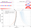 |
Figure 3 Eigenvalues of a system composed of a meter-long cylinder in the ω n − ζ n plane. The top plots show the modes shapes associated to each family: the trapped/resonator modes (left) and the exterior field modes (right). |
In Figure 3, we notice firstly that exterior modes have a relatively large damping compared to the resonator modes. Secondly, we note how their associated acoustic fields are localized in the exterior sphere. Strictly speaking, the distinction between resonator modes and exterior modes should be made with respect to the spatial distribution of their mode shapes W n (r, z). However, in our particular scenario, one can easily distinguish them through their location in the ω n − ζ n plane. Hence, a simple filtering mechanism is to set an appropriate limit value for the modal damping ζ n < ζ max , above which modes are considered “exterior" and hence discarded. Alternatively, one can also use an eigenvalue-based filter informed by the nature of exterior modes (acoustic modes of a spherical cavity in this case). For example, a heuristic choice that works well for various values of the sphere’s radius R, is to set
 (25)
(25)
where values for coefficient 1 < β < 4, typically work well. An example of this curve is illustrated as a thin-dotted line in Figure 3. This might seem trivial for the example shown in Figure 3 but it provides a robust approach for more general scenarios, where the eigenvalues of resonator modes might have a less regular behavior (as seen later in Fig. 5). Finally, Figure 3 illustrates well how viscothermal losses play a dominant role on the damping of the lower-order resonator modes. When frequency increases and wavelengths become comparable to the radius of the cylinder, we note that both models tend to similar damping values, indicating that radiation losses are dominant in higher-frequency modes, as expected.
4 Illustrative results on a simplified trumpet geometry
In this section, we present some illustrative numerical results on a simplified trumpet geometry made up of seven regular sections (cylindrical and conical). This geometry, introduced in [46], serves as a laboratory benchmark that is easy to prototype and approximates the bore geometry of a typical Bb trumpet, while avoiding issues related to confidential commercial information. Details of the considered geometry are presented in the upper table of Figure 4. For the numerical model, a wall thickness of 5 mm was considered (same as the prototype – described in the next section). The finite-element mesh was adapted according to the analysis performed. Namely, coarser meshes were used for linearized analysis where lower truncations N are reasonable while finer meshes were used for nonlinear analysis, where a larger number of modes needs to be considered for an accurate representation of nonlinear propagation phenomena. Two illustrative meshes are shown in Figure 4. Unless stated otherwise, the air properties used for the numerical results presented are shown in the lower table of Figure 4.
 |
Figure 4 Illustration of meshes used in the FE model. They lead to discretized systems with about 1000 and 10,000 degrees-of-freedom for the top and bottom examples, respectively, corresponding to maximal frequencies f max of about 1400 and 8000 Hz. |
4.1 Complex modal decomposition of simplified trumpet
Following the analysis presented previously, Figure 5 shows the distribution of the eigenvalues λ n stemming from the simplified trumpet model in the ω n − ζ n plane. These underline the key role of the viscothermal losses, which affect to a great degree the losses of the first ten modes. This is particularly important since these are the modes that will generally couple with the vibrating lips to generate self-sustained oscillations. It is interesting to note that the damping ratios of the trumpet modes with and without viscothermal losses remain almost “parallel" above the cut-off frequency, suggesting that the viscothermal losses have a persistent effect, even at very high frequencies. This is contrary to the simple cylinder example we have seen previously (Fig. 3), where radiation losses clearly dominate above a certain frequency. It is still unclear to us why exactly this occurs in the trumpet geometry, but it might be related to the small dimensions of the “throat" (narrowest part of the mouthpiece) and the larger localized viscothermal losses at this juncture.
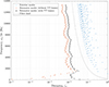 |
Figure 5 Distribution of eigenvalues, in the ω n − ζ n plane, resulting from the model of the simplified trumpet. Blue dots denote exterior modes, that are removed from the modal basis, red dots denote the eigenvalues from a system with radiation losses only and black dots the eigenvalues for a system with both radiation and viscothermal losses. |
Complex mode shapes are notably difficult to illustrate in a static image. This is because, contrary to the motion of real modes where all points move in unison, complex modes contain phase shifts between different spatial regions. Hence, while real modes represent standing wave patterns, complex modes are a combination of standing and travelling waves. They are generally represented by their real Re[W n (r, z)] and imaginary Im[W n (r, z)] parts separately. Moreover, complex modes are defined up to a multiplicative complex factor. In this case, it is often useful to “rotate" the complex mode by an angle β n (i.e., multiply by e −i β n ) such that it maximizes its real part. In this way, we can assess the “degree of complexity" of each mode by examining how large is its imaginary part. A simple way to find the optimal rotation angle β n * is given in [47], written here for discrete and continuous cases
 (26)
(26)
Figure 6 shows a few examples of the complex mode shapes W n (r, z) for the simplified trumpet model where the (maximized) real part is shown on the left-side and the (minimized) imaginary part on the right-side. Firstly, we note that the lower-order modes (n < 10) have a negligible imaginary part meaning they represent nearly standing waves and behave approximately as real normal modes. On the other hand, as frequency increases, we note an increasing “modal complexity". This relates to the fact that higher-frequency modes are mostly radiative, i.e., they essentially represent waves travelling through and out of the resonator. In simpler models, these high frequency modes are often neglected as they do not interact significantly with the lips (note their weak modal amplitudes near the mouthpiece). However, they play animportant role when attempting to accurately represent radiative behavior as well as nonlinear propagation.
Another benefit of modeling the exterior field is that, for example, the directivity of the trumpet at various (modal) frequencies can be assessed directly through the mode shapes themselves. That is, one can easily calculate the acoustic intensity at the radiative boundary Γ
r
in each complex mode shape  , hence obtaining an approximation of the far-field directivity at each modal frequency. Normalizing by the maximal absolute pressure one can obtain the modal directivity patterns via
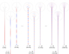 |
Figure 6 Complex mode shapes W n (r, z) of the simplified trumpet. The real and imaginary parts are represented in the left and right sides of each plot, respectively. Note: modes shapes were rotated such that their real part is maximized (imaginary part minimized). |
 (27)
(27)
where  pertains to the mode shape evaluated at the boundary Γ
r
and θ is the associated angle from the central axis. These are illustrated in Figure 7 for various modes in two different frequency ranges: < 4000 Hz (upper plot) and > 4000 Hz (lower plot).
pertains to the mode shape evaluated at the boundary Γ
r
and θ is the associated angle from the central axis. These are illustrated in Figure 7 for various modes in two different frequency ranges: < 4000 Hz (upper plot) and > 4000 Hz (lower plot).
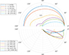 |
Figure 7 Modal directivity patterns D n (θ) for low/mid-range frequency modes (top) and high-frequency modes(bottom). |
We note how, at low frequencies (below 500 Hz), directivity patterns are nearly omnidirectional. This is expected since the associated wavelengths are much larger than the dimensions of the flaring horn. Between 1000 Hz and 4000 Hz, the directivity becomes much narrower, and relatively little acoustic energy is radiated behind the instrument’s horn. Here, the maximal values of the directivity remain on-axis. At very high frequencies however, when wavelengths are clearly smaller than the dimensions of the horn’s exit, directivity patterns can acquire rather complex patterns, with multiple lobes and maximal values that are not necessarily centered on-axis.
5 Experimental validation
Here we confront the results from the presented model to experimental measurements in both linear and nonlinear contexts involving harmonic forcing. The 7-cone trumpet is used as a test case geometry. For the experimental prototype, the long cylindrical section was made of brass piping while the conical parts were built using a resin stereolithography-based 3D printer, aimed to minimize rugosity on the inner surfaces (in contrast to filament-based printers).
5.1 Linear scenarios: input-impedance and radiation response
Regarding linear scenarios, two experimental tests were carried out on the simplified trumpet prototype to validate model results. Firstly, the input impedance of the trumpet was measured in a semi-anechoic chamber, using a CTTM impedance sensor [48]. Moreover, during the input-impedance measurements, a microphone was also placedoutside the flaring horn to measure its radiative response (transfer impedance). For the latter, three measurements were performed with the microphone placed at three different angles θ, and a constant distance of 100 mm from the center of the horn’s exit plane. These measurements allow for an indicative characterization of the horn’s directivity at various frequencies and highlight the role of higher-frequency modes, that are not observed in the input impedance measurements. Exponential sine sweeps, from 20 to 4000 Hz, were used to measure the input-impedance and the transfer impedance functions simultaneously.
Analogous model results were obtained via a modal description of a generic impedance transfer function relating a response pressure to a harmonic flow-rate excitation
 (28)
(28)
where over-bar denotes complex conjugation. For the input-impedance Z in(ω) in particular, the modal residues c n are given by [41]
 (29)
(29)
where Γ e pertains to the boundary of the mouthpiece entry. For a transfer impedance Z rad(ω), relating a pressure response at an exterior point (r ext, z ext) to a harmonic excitation at the mouthpiece, the residues are given by
 (30)
(30)
Modeled and measured results of the normalized input-impedance are shown in Figure 8, in terms of magnitude and phase. These illustrate the benefits of using a refined 2D-axisymmetric modeling framework and the motivation behind the current work as the modeled input-impedance is nearly a perfect fit to the measured results. An excellent correlation is seen even at higher frequencies, where commonly used 1D models may be less accurate, particularly when they are based on the assumption of plane waves.
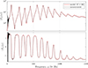 |
Figure 8 Measured and modeled normalized input impedance Z in(ω) of the simplified trumpet. Magnitude and phase are shown on the top and bottom, respectively. Model results were calculated using 15 modes. |
Experimental and model results for the transfer impedance functions are shown in Figure 9. As expected, responses for all microphones are quite similar at low frequencies with a slightly larger response on-axis. As already indicated in the directivity results, at higher frequencies, the response amplitude gradually decreases as one moves away from central axis. The model reproduces well the measured results, including the overall tendencies at higher frequencies as well as the small oscillations, product of the excitation of higher-frequency modes. Note that the latter effect can produce variations in response in the order of 4–5 dB SPL. Although small, this represents a non-negligible effect that emphasizes the role of higher order modes to the radiated sound and which is often neglected under the assumption of a flat response above the “cut-off" frequency. In the measured results, we also note an (unexpected) upwards drift of the overall tendency towards higher frequencies. Here, it must be noted that the actuator-cavity system in the CTTM impedance sensor has a resonant frequency around 5 kHz. Hence, these (slight) deviations might tentatively be attributed to an uneven response of the excitation system itself.
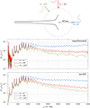 |
Figure 9 Experimental and modeled normalized radiative transfer functions for three microphone positions located at different angles with respect to the exit of the instrument. Here, modal truncation was set to N = 40. |
5.2 Nonlinear scenarios: large amplitude harmonic excitation
Subsequently, we aimed to assess the validity of the model in nonlinear, large amplitude scenarios. The conceived experimental set-up was aimed at exciting the trumpet prototype harmonically at its modal frequencies and examine the evolution of the (pseudo-)standing wave patterns when the excitation amplitude is increased, something that has not been previously presented in the context of musical instruments. Acoustic excitation was provided by dual-diaphragm compression driver (BMS 4599) placed at the entrance of the experimental prototype (this time without the embouchure, i.e., only the cylindrical section plus the bell). Note that this sort of set-up will inevitably influence the studied resonator since drivers have an non-negligible internal volume that is difficult to remove/reduce. For model validation purposes, this poses no problem since the internal volume can be taken into account in the model. However, naturally, the studied system in this case is not the same as the one described in the previous section.
The modal frequencies of the system were first identified via the exponential sine-sweep method at low amplitude. Subsequently, the system was excited at the various identified modal frequencies at increasing amplitudes. A pressure sensor (Endevco 8507C-5) was placed iteratively on 40 locations along the resonator’s length, aimed at giving a spatial illustration of the nonlinear standing wave patterns. Small holes (of 2.4 mm in diameter) were drilled alongside the resonator wall to fit the sensor tightly. A second reference pressure sensor was fixed inside the cavity of the compression chamber to get a phase reference. Signals from the pressure sensors were recorded at a sampling frequency of 96 kHz. It is worth noting that in the largest amplitudes measured, near shock wave behavior was observed, with spectral content clearly above 48 kHz.
Snapshots of the experimentally measured pressure fields inside the resonator when excited at different modal frequencies is shown in Figure 10, for small (blue) and large (red) amplitudes of excitation. The analogous results from the model (shown in the bottom of Fig. 10) were calculated via temporal integrations using a modal truncation of N = 100. An implicit scheme was used, namely, Matlab’s variable-order and variable-step ODE solver ode15i. Integrations were carried out for a fraction of a second (simulating about 0.3–0.4 s), until the system had reached a stable steady-state. For reference, computations generally took 1–5 min on a desktop computer with an Intel Core i9-13950HX (2.20 GHz) processor. Furthermore, to emulate experimental conditions, a cylindrical cavity was included at the entry of the model. The cavity dimensions (5 cm in height and 4 cm in radius) were roughly estimated based on a fit of measured and modeled modal frequencies (the lowest frequency being the most indicative, in this case at around 27 Hz).
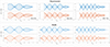 |
Figure 10 Snapshots of the measured (top) and modeled (bottom) on-axis pressure fields inside the resonator when excited at three modal frequencies at small (blue) and large (red) amplitudes. In the experimental results, dots denote the actual measurements while the connecting lines are a product of interpolation. Model results were calculated via temporal integrations where modal truncation was set to N = 100 and where the geometry was aimed at emulating the experimental configuration, i.e., including a cavity at the entrance (driver’s inherent volume). |
Results in Figure 10 show that standing wave pattern can be significantly deformed at large excitation amplitudes. As expected, we notice pressure fields with much steeper gradients. Curiously, we note a somewhat regular pattern whereby lobes near the open-end seem to be “rotated" clockwise while those near the closed-end counter-clockwise. Another important observation, that is not directly evident from the results in Figure 10, is that much steeper pressure gradients are found near the exit of the instrument compared to its entrance. This effect is seen clearly from the animated results presented in the supplementary material (“animated_trumpet_X.mp4”). Here, we note what seems to be a kind of superposition of a (slightly distorted) standing wave pattern and a travelling shock wave, or development thereof. This phenomena can interpreted from the point of view of localized radiation losses. That is, during motion, the cumulative nature of the nonlinear propagative terms will generate steep wavefronts. When these wavefronts reach the open-end of the instrument, most of their high-frequency content will be dissipated as radiation to the free field. In the context of harmonic forcing, this process of generation and extinction of steep wavefronts (or eventually shock waves) repeats periodically and, moreover, it is superimposed on the established standing wave pattern which retain most of the acoustic energy below the cut-off frequency (here at about 1–1.5 kHz).
From Figure 10, the model results seems to reproduce remarkably well the observed behavior, at least qualitatively. A closer look at the match between measured and modeled behavior in Figure 11, showing pressure signals at different locations along the resonator at different amplitudes (excitation at mode n = 8, 967.7 Hz). Overall, we retrieve the same temporal patterns for both the model and the experiment. Note that the small, noise-like oscillations in the large amplitude measurements are not “physical" but product of the sensor’s resonance (estimated around 50 kHz, but likely lower). This is likely the case since we have tested similar set-ups using different pressure sensors, resulting in perturbations with different dominant frequencies. Clearly, at these amplitudes, pressure sensors with higher resonance frequency are more adequate.
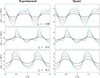 |
Figure 11 Temporal signals of the measured (left) and modeled (right) pressure at different locations along the resonator axis: z = −1.09 (top); z = −0.4 (center) and z = −0.1 (bottom), when excited at its 8th modal frequency (∼967.7 Hz) at different amplitudes. Time is here normalized by the period of the forcing frequency |

Aside from that, we also note a slight underestimation of the pressure gradients, indicating that, perhaps, the nonlinear propagation is underestimated by the model. This becomes clearer in Figure 12, showing the spectra corresponding to the signals in Figure 11. Firstly, we note the typical patterns of spectral enrichment, with higher harmonic content appearing with increasing amplitude. Secondly, we note that spectra of the modeled results drops-off abruptly above a certain frequency (red line), effectively corresponding to the frequency of the highest considered mode ωN. Clearly, the model cannot represent dynamics above this frequency limit. Note however that this does not necessarily mean that results are well approximated below this frequency, since the effects of modal truncation in nonlinear scenarios cannot be assured as in linear cases. Notably, we see that even below ωN the model slightly underestimates the experimental results. This underestimation could eventually be attributed to modal truncation errors. However, one must not forget that the nonlinear acoustics model also has its limits. As mentioned before, the range of validity for the Blackstock equation is estimated at about Mach number M < 0.1. Seen that we are clearly at very large amplitudes (discussing the eminence of shock waves in the experiments, i.e., M ∼ 1 locally), it is also possible that the Blackstock model has reached its limits and higher-order models would be necessary (e.g., Söderholm, see Eq. (1)). final note, it is worth mentioning that the accurate description of shock wave behavior in a modelling framework is a very ambitious task. In a modal framework, this would entail a very large (infinite in the conservative limit) modal truncation N. Similarly, in finite-element or finite-difference contexts, these would entail extremely fine meshes.
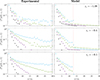 |
Figure 12 Normalized spectra of the periodic signals shown in Figure 11. Each marker denotes the magnitude of each harmonic component in the periodic signal, normalized by the magnitude of its first component. The red-dotted line denotes the frequency of the highest considered mode ω N . Frequency is here normalized by the forcing frequency ω 0. |
Nevertheless, overall, the model results were shown to approximate remarkably well the main features of the measured nonlinear behavior. With the exception of extreme cases, this illustrates how such models could be used reliably to characterize the timbre of real instruments with respect to their tendency (or otherwise) to generate nonlinear propagation.
6 Conclusion
Based on the second-order Blackstock equation for nonlinear acoustics and complex modal superposition, we presented in this work a framework that bridges the accuracy of 2D-axisymmetric models with the efficiency and compactness of reduced-order modal approaches. This allows one to build models including viscothermal losses, 2D radiation effects, the explicit calculation of radiated pressures as well as nonlinear propagation in large amplitude standing wave scenarios, at relatively low computational costs. Illustrative results for a simplified trumpet geometry are presented to clarify the procedures involved and the benefits of the proposed model are highlighted.
Experimental validation under harmonic forcing is performed in both linear and nonlinear scenarios. Overall, model results compare remarkably well with measured ones. In linear scenarios, both input- and transfer- (radiative) impedances are calculated with negligible errors. Similarly, under large amplitude forcing, the nonlinear model is able to accuratelyrepresent the distorted standing wave patters observed experimentally, despite a slight underestimation of nonlinear propagation effects at extreme amplitudes (near shock wave behavior). The latter point suggests the need for relatively large modal truncations and/or the use of higher-order nonlinear acoustics models.
The framework proposed here retains the same structure and efficiency of models typically used in musical acoustics while, at the same time, it can capture subtle features that are often missed by 1D models. Due to its relative compactness, these refined models are also compatible with heavier computational tasks like optimization, parametric studies, bifurcation analysis, etc. In a near future, we aim to use such models in more realistic playing conditions (including the coupling to a lip model) and study the effects of, among others, nonlinear propagation in the ensuing bifurcation diagrams (some preliminary studies have been published recently [49]).
Supplementary material
“animation_trumpet_1.mp4”: Animated experimentally measured pressure fields of the trumpet prototype excited harmonically at its 4th modal frequency (∼412.6 Hz). The blue and red curves reffer to excitations at small and large amplitudes, respectively. Access Supplementary Material
“animation_trumpet_2.mp4”: Animated experimentally measured pressure fields of the trumpet prototype excited harmonically at its 4th modal frequency (∼703.2 Hz). The blue and red curves reffer to excitations at small and large amplitudes, respectively. Access Supplementary Material
“animation_trumpet_3.mp4”: Animated experimentally measured pressure fields of the trumpet prototype excited harmonically at its 6th modal frequency (∼967.7 Hz). The blue and red curves reffer to excitations at small and large amplitudes, respectively. Access Supplementary Material
“animation_cylinder_1.mp4”: Animated experimentally measured pressure fields of a meter-long cylinder excited harmonically at its 4th modal frequency. Access Supplementary Material
“animation_cylinder_2.mp4”: Caption: Animated experimentally measured pressure fields of a meter-long cylinder excited harmonically at its 6th modal frequency. Access Supplementary Material
Conflicts of interest
I declare I have no conflict of interest.
Data availability statement
Data are available on request from the authors.
References
- A. Myers, J. Gilbert, M. Campbell: The science of brass instruments. Springer, 2021. [Google Scholar]
- S. Adachi, M.-A. Sato: Trumpet sound simulation using a two-dimensional lip vibration model. Journal of the Acoustical Society of America 99 (1996) 1200–1209. [CrossRef] [Google Scholar]
- A. Myers, R. Pyle, J. Gilbert, M. Campbell, J. Chick, S. Logie: Effects of nonlinear sound propagation on the characteristic timbres of brass instruments. Journal of the Acoustical Society of America 131, 1 (2012) 678–688. [Google Scholar]
- J. Chabassier, A. Thibault: Viscothermal models for wind musical instruments. INRIA, Project-Teams Magique 3D, 2020. [Google Scholar]
- P. Eveno, J.-P. Dalmont, R. Caussé, J. Gilbert: Wave propagation and radiation in a horn: comparison between models and measurements. Acta Acustica united with Acustica 98 (2012) 158–165. [Google Scholar]
- F. Silva, P. Guillemain, J. Kergomard, B. Mallaroni, A. Norris: Approximation formulae for the acoustic radiation impedance of a cylindrical pipe. Journal of Sound and Vibration 322 (2009) 255–263. [CrossRef] [Google Scholar]
- M. Campbell, J. Chick, J. Gilbert, J. Kemp, A. Myers, M. Newton: Spectral enrichment in brass instruments due to nonlinear sound propagation: a comparison of measurements and predictions. In: International Symposium on Musical Acoustics (ISMA), Le Mans, France, 2014. [Google Scholar]
- H. Berjamin, B. Lombart, C. Vergez, E. Cottanceau: Time-domain numerical modeling of brass instruments including nonlinear wave propagation, viscothermal losses and lip vibration. Acta Acustica united with Acustica 103, 2 (2017) 117–131. [CrossRef] [Google Scholar]
- S. Maugeais, J. Gilbert: Nonlinear acoustic propagation applied to brassiness studies, a new simulation tool in the time domain. Acta Acustica united with Acustica 103, 1 (2017) 67–79. [Google Scholar]
- F. Jensen, E. Brambley: Multimodal nonlinear acoustics in two- and three-dimensional curved ducts. arXiv, 2025. https://doi.org/10.48550/arXiv.2503.11536. [Google Scholar]
- R. Velasco-Segura, P. Rendón: Full-wave numerical simulation of nonlinear dissipative acoustics standing waves in wind instruments. Wave Motion 99 (2022) 102666. [Google Scholar]
- M. Berggren, A. Bernland, D. Noreland: Acoustic boundary layers as boundary conditions. Journal of Computational Physics 371 (2018) 633–650. [CrossRef] [Google Scholar]
- S. Krenk: Complex modes and frequencies in damped structural vibrations. Journal of Sound and Vibration 270 (2004) 981–996. [Google Scholar]
- S. Bilbao: Time domain simulations of brass instruments. In: Proceedings of Forum Acusticum, Aalborg, Denmark, 2011. [Google Scholar]
- N. Sugimoto: Burgers equation with a fractional derivative: hereditary effects on nonlinear acoustic waves. Journal of Fluid Mechanics 225, 1 (1991) 631–653. [Google Scholar]
- M. Ducceschi, C. Touzé: Modal approach for nonlinear vibrations of damped impacted plates: application to sound synthesis of gongs and cymbals. Journal of Sound and Vibration 344 (2015) 313–331. [Google Scholar]
- C. Issanchou, S. Bilbao, J.-L. L. Carrou, C. Touzé and O. Doaré: A modal-based approach to the nonlinear vibration of strings against a unilateral obstacle: Simulations and experiments in the pointwise case. Journal of Sound and Vibration 393 (2017) 229–251. [Google Scholar]
- P.M. Jordan: A survey of weakly-nonlinear acoustic models: 1910–2009. Mechanics Research Communications, vol. 73, pp. 127–139, 2016. [Google Scholar]
- L. Söderholm: A higher-order acoustic equation for the slightly viscous case. Acta Acustica 87 (2001) 29–33. [Google Scholar]
- D. Blackstock: Approximate equations governing finite-amplitude sound in thermoviscous fluids. General Dynamics Corporation, 1963. [Google Scholar]
- V. Kuznetsov: Equations of nonlinear acoustics. Soviet Physics – Acoustics 16 (1971) 467–470, 1971. [Google Scholar]
- B. Kaltenbacher, M. Meliani, V. Nikolić: The Kuznetsov and Blackstock equations of nonlinear acoustics with nonlocal-in-time dissipation. Applied Mathematics & Optimization 89 (2024) 63. [Google Scholar]
- B. Kaltenbacher, R. Brunnhuber: Nonlinear Acoustics. Snapshots of Modern Mathematics From Oberwolfach 8 (2019) 1–12. [Google Scholar]
- S. Makarov, M. Ochmann: Nonlinear and thermoviscous phenomena in acoustics. Acustica 83 (1997) 197–222. [Google Scholar]
- S. Félix, J.-P. Dalmont, C.J. Nederveen: Effects of bending portions of the air column on the acoustical resonances of a wind instrument. Journal of the Acoustical Society of America 131 (2012) 4164–4172. [Google Scholar]
- A. Sommerfeld: Die Greensche Funktion der Schwingungslgleichung. Jahresbericht der Deutschen Mathematiker-Vereinigung 21 (1912) 309–352. [Google Scholar]
- L. Thompson: A review of finite-element methods for time-harmonic acoustics. Journal of the Acoustical Society of America 119, 3 (2006) 1315–1330. [Google Scholar]
- J. Shirron, I. Babuska: A comparison of approximate boundary conditions and infinite element methods for exterior Helmholtz problems. Computer Methods in Applied Mechanics and Engineering 164, 1 (1998) 121–139. [Google Scholar]
- A. Bayliss, M. Gunzburger, E. Turkel: Boundary conditions for the numerical solution of elliptic equations in exterior regions. SIAM Journal of Applied Mathematics 42, 1 (1982) 430–451. [Google Scholar]
- M. Mikhail, M. El-Tantawy: The acoustic boundary layers: a detailed analysis. Journal of Computational and Applied Mathematics 51 (1994) 15–31. [Google Scholar]
- A. Hirschberg, J. Gilbert, R. Msallam, P. Wijnands: Shock waves in trombones. Journal of the Acoustical Society of America 99 (1996) 1754–1758. [CrossRef] [Google Scholar]
- A. Ernoult, J. Kergomard: Transfer matrix of a truncated cone with viscothermal losses: application of the WKB method. Acta Acustica 4 (2020) 11. [Google Scholar]
- G. Everstine: Finite element formulations of structural acoustics problems,” Computers & Structures. 65, 3 (1997) 307–321. [Google Scholar]
- P. Rucz, J. Chabassier: Examination of computational models of weakly nonlinear sound propagation in ducts. In: DAGA 2024, Hannover, Germany, 2024. [Google Scholar]
- S. Adhikari: Damping models for structural vibration. PhD Thesis, Cambridge University Engineering Department, 2000. [Google Scholar]
- M. Grohlich, M. Boswald, R. Winter: An iterative eigenvalue solver for systems with frequency dependent material properties. In: DAGA 2020, Hannover, Germany, 2024. [Google Scholar]
- J. Woodhouse: Linear damping models for structural vibration. Journal of Sound and Vibration 215, 3 (1998) 547–569. [Google Scholar]
- Y. Saad: Numerical methods for large eigenvalue problems: revised edition. Society for Industrial and Applied Mathematics (SIAM), Philadelphia, 2011. [Google Scholar]
- T. Caughey, M. O’Kelly: Classical normal modes in damped linear dynamic systems. Journal of Applied Mechanics 32 (1965) 583–588. [Google Scholar]
- L. Li, Y. Hu, W. Deng, L. Lü, Z. Ding: Dynamics of structural systems with various frequency-dependent damping models. Frontiers in Mechanical Engineering 10 (2015) 48–63. [Google Scholar]
- F. Ablitzer: Peak-picking identification technique for modal expansion of input impedance of brass instruments. Acta Acustica 5 (2021) 53. [CrossRef] [EDP Sciences] [Google Scholar]
- S. Adhikari, J. Woodhouse: Quantification of non-viscous damping in discrete linear systems. Journal of Sound and Vibration 260 (2003) 499–518. [Google Scholar]
- F. Soares, C. Vergez, V. Freour, B. Cochelin, “Modal approaches for linear and nonlinear dynamical systems with non-classical damping“, Journal of Sound and Vibration, vol. 618 (B), 119352, 2025. [Google Scholar]
- Z. Xintao, Z. Yaobing, C. Shaohui, G. Zhirui: Effects of mode truncation on nonlinear coupled resonant responses of suspended cable. Journal of Vibration and Shock 42, 3 (2023) 50–56. [Google Scholar]
- S. Marburg: Normal modes in external acoustics. Part I: Investigation of the one-dimensional duct problem. Acta Acustica united with Acustica 91 (2005) 1063–1078. [Google Scholar]
- B. Cochelin, V. Freour, C. Vergez: Exploiting the use of strong nonlinearity in dynamics and acoustics: the case of musical wind instruments, Vol. 613, CISM, Springer, Cham, (2024) pp. 121–149. [Google Scholar]
- P. Vacher, B. Jacquier, A. Bucharles: Extensions of the MAC criterion to complex modes. In: Proceedings of ISMA2010, Leuven, Belgium, 2010. [Google Scholar]
- J.-P. Dalmont, J.C.L. Roux: Capteur d’impédance. Centre de Transfer de Technologie du Mans (CTTM). Available at https://www.cttm-lemans.com/fr/acoustique-vibrations/produits/capteur-d-impedance.html. [Google Scholar]
- F. Soares, V. Fréour, B. Cochelin, C. Vergez, K. Arimoto: Bifurcation diagrams of a brass instrument model including nonlinear acoustic propagation. In: Proceedings of Meetings on Acoustics (ISMRA), New Orleans, 2025. [Google Scholar]
Cite this article as: Soares F. Cochelin B. Freour V. Vergez C. & Arimoto K. 2025. Nonlinear acoustics in brass instruments using 2D complex modal bases. Acta Acustica 9, 68. https://doi.org/10.1051/aacus/2025049.
All Figures
|
Figure 1 Illustrative scheme of the proposed modeling approach: (1) discretize 2D linear problem via FE model; (2) compute the complex modal basis from the associated quadratic eigenvalue problem; (3) projection of nonlinear acoustics PDE onto complex modal basis. |
| In the text | |
|
Figure 2 Diagram of the considered axisymmetric model. The dashed and dash-dotted lines correspond to the viscothermal Γ v t and radiative Γ r boundaries, respectively. |
| In the text | |
|
Figure 3 Eigenvalues of a system composed of a meter-long cylinder in the ω n − ζ n plane. The top plots show the modes shapes associated to each family: the trapped/resonator modes (left) and the exterior field modes (right). |
| In the text | |
|
Figure 4 Illustration of meshes used in the FE model. They lead to discretized systems with about 1000 and 10,000 degrees-of-freedom for the top and bottom examples, respectively, corresponding to maximal frequencies f max of about 1400 and 8000 Hz. |
| In the text | |
|
Figure 5 Distribution of eigenvalues, in the ω n − ζ n plane, resulting from the model of the simplified trumpet. Blue dots denote exterior modes, that are removed from the modal basis, red dots denote the eigenvalues from a system with radiation losses only and black dots the eigenvalues for a system with both radiation and viscothermal losses. |
| In the text | |
|
Figure 6 Complex mode shapes W n (r, z) of the simplified trumpet. The real and imaginary parts are represented in the left and right sides of each plot, respectively. Note: modes shapes were rotated such that their real part is maximized (imaginary part minimized). |
| In the text | |
|
Figure 7 Modal directivity patterns D n (θ) for low/mid-range frequency modes (top) and high-frequency modes(bottom). |
| In the text | |
|
Figure 8 Measured and modeled normalized input impedance Z in(ω) of the simplified trumpet. Magnitude and phase are shown on the top and bottom, respectively. Model results were calculated using 15 modes. |
| In the text | |
|
Figure 9 Experimental and modeled normalized radiative transfer functions for three microphone positions located at different angles with respect to the exit of the instrument. Here, modal truncation was set to N = 40. |
| In the text | |
|
Figure 10 Snapshots of the measured (top) and modeled (bottom) on-axis pressure fields inside the resonator when excited at three modal frequencies at small (blue) and large (red) amplitudes. In the experimental results, dots denote the actual measurements while the connecting lines are a product of interpolation. Model results were calculated via temporal integrations where modal truncation was set to N = 100 and where the geometry was aimed at emulating the experimental configuration, i.e., including a cavity at the entrance (driver’s inherent volume). |
| In the text | |
|
Figure 11 Temporal signals of the measured (left) and modeled (right) pressure at different locations along the resonator axis: z = −1.09 (top); z = −0.4 (center) and z = −0.1 (bottom), when excited at its 8th modal frequency (∼967.7 Hz) at different amplitudes. Time is here normalized by the period of the forcing frequency |
| In the text | |
|
Figure 12 Normalized spectra of the periodic signals shown in Figure 11. Each marker denotes the magnitude of each harmonic component in the periodic signal, normalized by the magnitude of its first component. The red-dotted line denotes the frequency of the highest considered mode ω N . Frequency is here normalized by the forcing frequency ω 0. |
| In the text | |
Current usage metrics show cumulative count of Article Views (full-text article views including HTML views, PDF and ePub downloads, according to the available data) and Abstracts Views on Vision4Press platform.
Data correspond to usage on the plateform after 2015. The current usage metrics is available 48-96 hours after online publication and is updated daily on week days.
Initial download of the metrics may take a while.