| Issue |
Acta Acust.
Volume 9, 2025
|
|
|---|---|---|
| Article Number | 80 | |
| Number of page(s) | 15 | |
| Section | Aeroacoustics | |
| DOI | https://doi.org/10.1051/aacus/2025064 | |
| Published online | 09 January 2026 | |
Scientific Article
A quasi-one-dimensional critical-throat acoustic boundary condition for thermally choked dual-mode ramjet nozzles
1
DMPE, ONERA, Université Paris-Saclay, Palaiseau, 91120, France
2
DMPE, ONERA, Université de Toulouse, Toulouse, 31000, France
3
Department of Applied Physics, Technische Universiteit Eindhoven, Eindhoven, 5600 MB, The Netherlands
* Corresponding author: This email address is being protected from spambots. You need JavaScript enabled to view it.
Received:
24
July
2025
Accepted:
14
November
2025
Abstract
Thermally choked nozzles, where choking is induced by heat addition rather than a geometrical throat, are a promising solution for dual-mode ramjet transitions to hypersonic speed. Despite their relevance, thermal throat boundary conditions for quasi-one-dimensional acoustic modelling are not derived in the state-of-the-art. This study introduces a generalized critical-throat acoustic boundary condition applicable to both geometrically and thermally choked flow configurations. A dedicated one-dimensional linear acoustic solver is formulated to incorporate this condition and is validated against two-dimensional Euler simulations. Particular attention is paid to the impact of entropy and acoustic waves at the critical throat. The results show that the new boundary condition improves the prediction of acoustic reflection, entropy noise production, and transmission coefficients, especially under thermally choked conditions where the commonly used quasi-steady assumption fails. For both the thermal-throat and geometric-throat configurations, the deviation in the acoustic transmission coefficient between the linear acoustic model using the proposed boundary condition and the simulations remains below 2%, while the deviation in the entropy-noise transmission coefficient remains below 5%, demonstrating the robustness of the proposed boundary condition.
Key words: Dual-mode ramjet / Thermal throat / Linear model / Acoustic / Entropy
© The Author(s), Published by EDP Sciences, 2025
 This is an Open Access article distributed under the terms of the Creative Commons Attribution License (https://creativecommons.org/licenses/by/4.0), which permits unrestricted use, distribution, and reproduction in any medium, provided the original work is properly cited.
1 Introduction
Ramjets and scramjets are key propulsion systems for high-speed flight due to their higher propulsive efficiency compared to turbojets and turbofans at equivalent velocities. Ramjets operate with subsonic combustion and are effective up to moderate flight Mach numbers (Mach 5), but their performance deteriorates at higher speeds due to substantial pressure losses and the effects of chemical dissociation and recombination [1]. In contrast, scramjets use supersonic combustion, achieving greater efficiency at Mach numbers above 5, making them suitable for hypersonic air breathing applications [2]. To extend operability across a wider range of Mach numbers in flight, dual-mode ramjets have been developed. These engines can seamlessly shift between the subsonic and supersonic combustion regimes, offering adaptability in a wide range of flight conditions [3, 4]. However, this versatility introduces significant design complexity.
In conventional ramjets, a geometric throat is used to choke the flow, hereafter referred to as a geometrically choked-flow nozzle. Although effective in low-flight Mach number combustion regimes, this configuration becomes unsuitable under scramjet conditions. An alternative is the use of a thermal throat (Fig. 1), produced by the volumetric heat release from combustion [5, 6]. Unlike the geometric configuration, this design uses a purely divergent nozzle, enabling a continuous transition between combustion regimes without altering the geometry of the engine.
 |
Figure 1. Sketch of an idealized dual-mode ramjet incorporating a thermal throat. |
Quasi-one-dimensional linear acoustic models are powerful tools for analysing and designing the acoustic behaviour of combustion chambers due to their numerical efficiency. However, they involve a one-dimensional acoustic boundary condition at the critical-throat location. For example, Lin et al. [7] proposed a model that describes the acoustic feedback loop in a scramjet combustor featuring a thermal throat, but treated the flame and critical throat as a single acoustic boundary, thus neglecting their distinct physical roles.
In quasi-one-dimensional acoustic models, it is commonly assumed that Mach number fluctuations vanish at the critical throat [8–13]. While this assumption holds under quasi-steady, isentropic flow conditions for geometrically choked nozzles, Olivon et al. [14, 15] demonstrated its failure under unsteady inlet conditions for both geometrical and thermal throats. In particular, this quasi-steady critical Mach number assumption induces a singularity at the critical-throat location [15]. Building on the work of Marble and Candel [8], a generalized boundary condition has been proposed for isentropic flows [15]. The key idea behind this theory is to impose a regular solution for the acoustic field at the throat. This was originally proposed by Tsien [16], following a suggestion by Crocco, and later used by Marble and Candel [8] for a particular nozzle geometry. Considering a series expansion of the solution in powers of the distance from the critical throat, Tsien [16] discarded the solution whose leading-order term is inversely proportional to that distance. A generalization of this approach for thermally choked configurations is proposed in the present study.
The effect of heat addition on flow dynamics has been extensively studied in subsonic flows, particularly in the context of acoustic wave propagation. These studies show that steady heating can induce acoustic absorption [17, 18] and generate entropy waves as acoustic waves propagated through the heated region [19–21]. Beyond the subsonic regime, investigations have focused on geometrically choked flows, providing important insights into aero-acoustic responses and wave dynamics [22–25]. However, none of these studies have addressed heat addition as the primary choking mechanism.
All the aforementioned works assume a calorically perfect gas, in which the specific heat capacities are considered temperature-independent and the flow is assumed to be isentropic. However, in thermally-choked flows, characterized by significant temperature variations, theses assumptions are inherently questionable [26–28]. Olivon et al. [14] numerically investigated the impact of temperature-dependent specific heat capacities and demonstrated that both the acoustic-reflection and entropy-noise-production coefficients can vary by as much as 20%. These findings indicate that the heat capacity temperature dependency must be taken into account to model thermally-choked flows using linear acoustic models.
In the present work, the inviscid assumption is used which is common in the literature on geometrical-throat nozzles [8, 10, 13], because boundary layers are thin. Although these layers modify the mean central flow, their influence on thermal throat dynamics has been shown to be limited [29]. The volumetric heat source term P v is assumed to be steady, and fluctuations in heat release are not considered. This implies no feedback loop between the heat release and flow field, as adopted in previous studies [17, 22, 30]. Yeddula et al. [31] highlighted this model limitation; nevertheless, it allows for a first step before introducing more complex phenomena. Finally, the analysis is limited to acoustic and entropy waves; indirect noise arising from gas mixture non-uniformity, as investigated by Gentil et al. [13, 32], is not taken into account.
The objective of this study is to develop and validate a boundary condition that describes the behaviour of the critical throat subjected to both acoustic and entropy wave forcing in a thermally choked flow configuration. The quasi-one-dimensional linear acoustic model employed is validated against two-dimensional Euler numerical simulations.
The paper is organized as follows. The quasi-one-dimensional linear acoustic model is first presented in Section 2, along with the new critical throat boundary condition model in Section 3. The methodology and numerical parameters used for the validation of the proposed boundary condition are then introduced in Section 4. Results and discussions follow in Section 5. Conclusions are summarized in Section 6.
2 Quasi-one-dimensional linear acoustic model
The following assumptions define the limits of validity of the present model. First, the flow is modelled as quasi-one-dimensional, and only plane waves are considered. Second, the Euler equations are employed, neglecting viscous and thermal diffusion effects. Third, a non-uniform, steady volumetric heat source term P v is introduced to model the energy release from the flame. The influence of the acoustic perturbations on this heat release are neglected.
2.1 Flow model
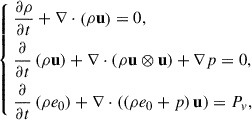
For an ideal gas, assuming no losses due to viscosity, thermal diffusion, or external force fields, the standard quasi-one-dimensional equations for mass, momentum, and energy conservation are expressed as follows [8]:
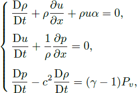 (1)
(1)
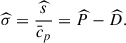
where D/Dt = ∂/∂t + u ∂/∂x is the material derivative, ρ is the density, u is the longitudinal velocity, α = (dA/dx)/A is the relative variation of the nozzle cross-sectional area A, p is the static pressure, c is the speed of sound, γ = c p /c v is the ratio of specific heats at constant pressure c p and constant volume c v , and P v is the volumetric heat-rate addition source term. For clarity and conciseness, the system of equations (1) will hereafter be referred to as the quasi-one-dimensional Euler equations.
To close the quasi-one-dimensional Euler equations (1), the ideal gas law is used:
 (2)
(2)
where T is the static temperature, r = ℛ/𝒲 is the specific gas constant, with ℛ = 8.3145 J mol−1K−1 the universal gas constant, and 𝒲 the molar mass of the gas.
The gas considered here is the air, described as an ideal gas with a specific isobaric heat capacity c p , function of the temperature. It is computed using a seventh-order polynomial function of the static temperature T:
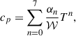 (3)
(3)
where α n are the heat capacity coefficients provided by Lemmon et al. [33].
For a uniform gas composition, the Gibbs energy equation provides a relation between the variations of entropy s, temperature T and pressure p such as:
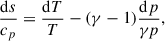 (4)
(4)
for a reversible process.
2.2 Linear acoustic propagation model
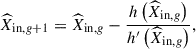
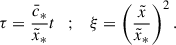
To study the propagation of acoustic and entropy waves through an heated nozzle with non-uniform steady flow field, quasi-one-dimensional Euler equations (1) are linearized using the perturbation convention  , where
  denotes the steady component and y′ the small perturbation of y = [ρ, u, p, T, c, γ]. The volumetric heat-rate source term P
v
being prescribed as steady, there are no fluctuations (P
v
′=0). Neglecting second-order perturbations and introducing the normalized quantities
denotes the steady component and y′ the small perturbation of y = [ρ, u, p, T, c, γ]. The volumetric heat-rate source term P
v
being prescribed as steady, there are no fluctuations (P
v
′=0). Neglecting second-order perturbations and introducing the normalized quantities  ,
,  ,
,  yields the following linearized system of differential equations:
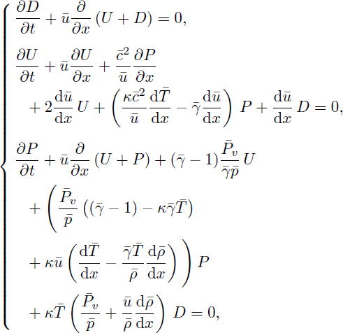 (5)
(5)
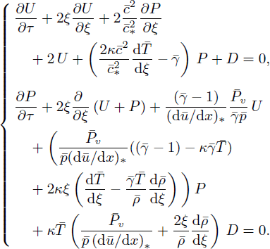
where  is the relative isentropic ratio variation. This system is an extension to heated and non-isentropic flow of the Linearized Euler Equations (LEE) system described in [8, 10, 13].
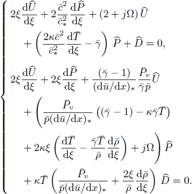
Assuming a mono-frequency forcing, the linearized quasi-one-dimensional Euler system equation (5) is rewritten using the convention  , where
  is the complex amplitude of the Fourier transform of the quantity y, and ω = 2π
f is the angular frequency. Introducing the unknown vector
is the complex amplitude of the Fourier transform of the quantity y, and ω = 2π
f is the angular frequency. Introducing the unknown vector 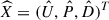 leads to the following matrix equation:
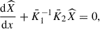 (6)
(6)
with
where  is the steady-flow Mach number, and
 (7)
(7)
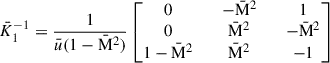
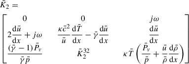
where the matrix coefficient  is given by:
 (8)
(8)
It is noteworthy that  is invertible if and only if
  and
and  as pointed out by Duran and Moreau [10]. This implies that the present acoustic model is not valid at the sonic (critical) throat.
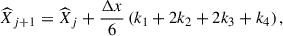
Introducing the matrix  and assuming a discretization of the nozzle over j ∈ ⟦0, …, l − 1, l, l + 1, …, n⟧ elements (the index l denotes the critical-throat position), each of size Δx, and using an explicit fourth-order Runge–Kutta (RK4) numerical scheme [34] for integration, the following relation is obtained:
 (9)
(9)
with the intermediate slopes defined as, ∀j ≠ l:
To ensure convergence of the solution, a Newton–Raphson root-finding method is employed to impose a continuity condition at the critical-throat location (see Sect. 3).
2.3 Waves decomposition and acoustic coefficients
The acoustic and entropy waves propagating through the flow are introduced via the inlet boundary conditions (see Sect. 3) and are used to solve the system equation (6). However, although the system is solved for the fluctuations  ,
,  , and
, and  along the spatial domain x, these variables do not directly correspond to pure acoustic or entropy plane waves. Therefore, a wave decomposition is required.
In a region of uniform flow, the acoustic pressure field can be decomposed into downstream- ( ) and upstream-propagating (
 ) wave components using the following relations:
 (10)
(10)
Such a uniform flow region is assumed both upstream and downstream of the nozzle (i.e., at the inlet and the outlet), as detailed in Figure 2.
 |
Figure 2. Sketch of the boundary condition treatment for a thermally choked flow configuration. A similar decomposition can be applied to a nozzle with a geometric throat. |
The linearized entropy fluctuation is defined as  , which, in the frequency domain and according to the Gibbs energy equation (4), becomes:
 (11)
(11)
Since entropy disturbances are convected with the mean flow  , they propagate in the downstream direction.
Based on the decomposition into downstream- and upstream-propagating plane waves, the reflection and transmission coefficients can be defined. For isentropic acoustic waves, the inlet acoustic reflection coefficient R a is defined as the ratio of the upstream- to downstream-propagating acoustic wave amplitudes at the inlet (subscript “in”):
 (12)
(12)
The acoustic transmission coefficient T a is defined as the ratio of the downstream-propagating isentropic acoustic wave amplitudes at the outlet (subscript “out") and inlet:
 (13)
(13)
Similarly, the entropy-noise production coefficient R
s
is defined as the ratio of the upstream-propagating isentropic acoustic wave to the incoming entropy wave for a vanishing incoming acoustic wave ( ):
):
 (14)
(14)
and the entropy-noise transmission coefficient T s is the ratio of the downstream-propagating isentropic wave at the outlet to the entropy wave at the inlet:
 (15)
(15)
It is noteworthy that this definition of the transmission coefficient assumes that the flow is uniform and non-heated at the outlet of the geometry. Consequently, the coefficient depends on the specific location where the outlet quantities are measured. This coefficient is primarily used to validate the supersonic region of the quasi-one-dimensional linear acoustic model.
3 Boundary conditions
To solve equation (6), three boundary conditions must be applied at the system boundaries. Following the methodology of Duran and Moreau [10], the unknown vector  is computed in two stages (see Fig. 2).
In the subsonic region, two boundary conditions must be applied at the inlet (x in), and one at the upstream side of the critical-throat (denoted x cu).
To ensure that the system equation (6) remains invertible ( ), the locations where boundary conditions are applied near the critical throat are shifted slightly away from the sonic point by an infinitesimal distance ϵ, as illustrated in Figure 2, leading to x
cu = x
* − ϵ and x
cd = x
* + ϵ. This distance ϵ is set equal to the spatial discretization Δx.
), the locations where boundary conditions are applied near the critical throat are shifted slightly away from the sonic point by an infinitesimal distance ϵ, as illustrated in Figure 2, leading to x
cu = x
* − ϵ and x
cd = x
* + ϵ. This distance ϵ is set equal to the spatial discretization Δx.
As only two boundary conditions are imposed at the inlet, a root-finding method must be employed to determine the third component of the unknown vector  . For instance,
  and
and  are prescribed as input values, while the third component
  is initially guessed, forming the inlet unknown vector
  . The linear acoustic model equation (9) is then used to compute the spatial profiles of
  ,
,  , and
, and  .
.
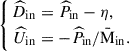
At the critical-throat position x
cu, the corresponding boundary condition (which will be detailed in Sect. 3.2) is evaluated as a root function, denoted  . Based on the outcome, the guessed inlet condition is updated using the Newton–Raphson method:
 (16)
(16)
where the derivative  is approximated using a first-order explicit finite-difference scheme.
To ensure convergence of the root-finding method, the relative error on the critical-throat boundary condition is set to 1 × 10⁻⁸. The initial guess of the unknown vector is based on an isentropic downstream-propagating acoustic wave for acoustic forcing and downstream-propagating entropy wave for entropy forcing. It has been verified that this initial guess does not affect the final value of  .
.
Subsequently, the supersonic region is solved by imposing three boundary conditions just downstream of the critical-throat position, denoted x
cd and no conditions at the outlet  . The resulting solution satisfies the continuity condition
  .
.
3.1 Inlet boundary conditions
For an isentropic acoustic forcing of angular frequency ω = 2π
f, the inlet acoustic pressure fluctuation  is imposed with an amplitude η. As the forcing is assumed to be perfectly isentropic, i.e.,
  , the following inlet boundary conditions apply:
 (17)
(17)
For entropy forcing of angular frequency ω, an entropy amplitude η is applied at the inlet, and the downstream-propagating acoustic wave is set to zero, i.e., 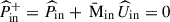 , resulting in the following two inlet boundary conditions:
 (18)
(18)
3.2 Critical-throat acoustic-boundary condition
In the literature [8–13], a commonly used approach is the quasi-steady critical Mach number assumption, which states that Mach number fluctuations vanish at the steady critical-throat position, i.e., M′* = 0. The subscript ()* hereafter denotes quantities evaluated at the steady critical-throat location. For isentropic gas flows with constant heat capacity ratio γ, this quasi-steady critical-throat boundary condition (denoted QSS) can be expressed as:
 (19)
(19)
Using the linearized Gibbs equation ((Eq. 11)), the entropy-based form of this condition, as given by Marble and Candel [8] and Duran and Moreau [10], becomes:
 (20)
(20)
However, it has been shown in previous works [15, 26] that the critical-throat position is not steady under acoustic and entropy mono-harmonic plane wave forcing, and that the quasi-steady assumption does not hold, even for isentropic nozzles (except at very low frequencies). In what follows, a new boundary condition is proposed for thermally-choked-flows.
As performed by Tsien [16] and Marble and Candel [8], the steady flow velocity profile,  , is locally approximated at the throat as
  , where
  denotes the velocity gradient at the critical-throat. The origin of the coordinate
  is chosen such that the extrapolated velocity profile
  vanishes at
  . The throat position is
  . Based on this definition, the following time-space transformation is introduced as performed by Marble and Candel [8]:

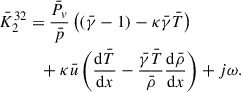
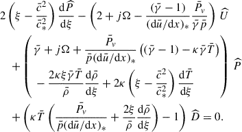
This boundary condition is based on the linearized quasi-one-dimensional Euler equations (5), rewritten using the above time-space transformation. Introducing the dimensionless frequency  , the system equation (5) is further expressed in the frequency domain. This dimensionless frequency characterizes how the critical throat interacts with the propagating waves through the local velocity gradient. The condition is derived by subtracting the energy equation from the momentum equation (see Appendix A for details). The assumption of Tsien [16], as proposed by Crocco, is adopted such that
  ,
,  , and
, and  , as well as their derivatives, are continuous at the critical-throat location. It is further assumed that none of the leading-order terms in the expansion of these quantities is proportional to 1/(1 − ξ). Such a condition would lead to a singularity at the critical throat. Under these assumptions, and because at the throat ξ = 1,
  and terms in ξ − 1 vanish, the generalized boundary condition at the critical-throat position (denoted GEN) becomes:
 (21)
(21)
where the coefficients are defined as:
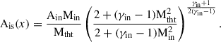
![Mathematical equation: $$ \begin{aligned} \left\{ \begin{aligned} \bar{g}_{U}&= 2 + j\mathrm{\Omega } - \dfrac{\left(\bar{\gamma }_* - 1\right)}{\left(\mathrm{d} \bar{u}/\mathrm{d} x\right)_*} \dfrac{\bar{P}_{v,*}}{\bar{\gamma }_* \bar{p}_*}, \\ \bar{g}_P&= \bar{\gamma }_* + j\mathrm{\Omega } + \dfrac{\bar{P}_{v,*}}{\bar{p}_*\left(\mathrm{d} \bar{u}/\mathrm{d} x\right)_*} \\&\quad \left[ \left(\bar{\gamma }_* - 1\right) - \kappa _* \bar{\gamma }_* \bar{T}_* \right] - \dfrac{2 \kappa _* \bar{\gamma }_* \bar{T}_*}{\bar{\rho }_*} \left. \dfrac{\mathrm{d} \bar{\rho }}{\mathrm{d} \xi } \right|_*, \\ \bar{g}_D&= \kappa _* \bar{T}_* \left( \dfrac{\bar{P}_{v,*}}{\bar{p}_*\left(\mathrm{d} \bar{u}/\mathrm{d} x\right)_*} + \dfrac{2}{\bar{\rho }_*} \left. \dfrac{\mathrm{d} \bar{\rho }}{\mathrm{d} \xi } \right|_* \right) - 1. \end{aligned} \right. \end{aligned} $$](/articles/aacus/full_html/2025/01/aacus250104/aacus250104-eq78.gif) (22)
(22)
This critical-throat boundary condition is an extension of the boundary condition for isentropic flow proposed by Olivon et al. [15], to heated and non-calorically perfect gas flows. Further details on the derivation of this model are provided in Appendix A.
The asymptotic behaviour of this boundary condition is also of interest. At very high frequencies (Ω ≫ 1), the relation  emerges, indicating that in a heated medium, the generation of entropy due to propagating acoustic waves becomes negligible. This is because
  becomes negligible compared to
  . Furthermore, this relation suggests that acoustic reflection at the critical throat vanishes, and the boundary condition can be approximated at high frequencies by an isentropic, non-reflective boundary condition.
As explained previously, at the critical-upstream position x cu the boundary condition is evaluated as a root function. Depending on whether the quasi-steady (QSS) or the generalized formulation (GEN) is chosen, it writes:
 (23)
(23)
 (24)
(24)
4 Validation methodology
To validate the GEN boundary condition proposed in equation (21), results from the quasi-one-dimensional acoustic model using this boundary condition ((Eq. 6)) are compared with two-dimensional Computational Fluid Dynamics (CFD) simulations. These simulations are conducted at low amplitudes, with η = 1 × 10⁻², ensuring that a linear unsteady-perturbation propagation is expected. Two choking configurations are investigated: an isentropic geometric-throat configuration and a thermally-choked-flow configuration. The results comparisons are performed on the acoustic coefficients (R a , R s , T a and T s ) previously defined in Section 2.3.
In the following, only the main steps of the methodology are outlined.
4.1 Thermally choked flow nozzle
For the thermally-choked flow configuration, a simplified dual-mode ramjet geometry, based on the works of [6, 14, 26, 28], is used, as shown in Figure 3. The nozzle geometry consists of three sections: a straight-duct upstream section (0 ≤ x/L < xu/L = 0.42), a smooth transition section (xu/L = 0.42 ≤ x/L < xd/L = 0.58) formed by a wall in circular arc with angle α = 3°, and a divergent duct with a constant divergence angle α = 3° (x/L > xd/L = 0.58). The total length and inlet height of the nozzle are L = 2.4 m and yin = 25 × 10−3 m, respectively. The circular arc radius of the transition region is Rt/yin = 305. A slip-adiabatic boundary condition is imposed on the upper nozzle wall, while a symmetry boundary condition is applied along the lower edge.
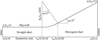 |
Figure 3. Simplified two-dimensional planar sketch of a dual-mode ramjet geometry (not to scale). |
The incoming airflow at the inlet is subsonic, as detailed in Table 1. The inlet conditions are representative of typical dual-mode ramjet engine operation [6].
Nozzle-inlet Mach number Min, total temperature T 0, in, and static pressure p in, corresponding to a typical flight Mach number M = 3.
To establish a steady thermal throat deep within the divergent nozzle via non-uniform heat release, the approach from prior works [14, 26, 28] is adopted. The spatial distribution of P v (x) is divided into two regions. In the straight duct (Fig. 3), the flow is not heated, P v is set to zero. In the divergent section (x > x u), the volumetric power distribution P v follows a log-normal profile along x, as proposed by Wang et al. [4] and Olivon et al. [14].
To determine P v (x), a quasi-one-dimensional steady-state model is used, based on the Mach number and static temperature formulations by Shapiro [35] for an ideal gas, and the steady-state thermal throat relation of Heiser and Pratt [36]. This model does not directly define P v (x). It determines the gradient of the heat release per unit mass, dq/dx:
 (25)
(25)
where  is the quasi-one-dimensional steady mass flow rate, calculated using isentropic relations and the inlet conditions provided in Table 1. The model is tuned to achieve a steady-state thermal throat located at x
*/L = 0.8, corresponding to a flame length of (x
* − x
u)/L = δ
*/L = 0.38. This location aligns with the mean spatial position of the thermal throat in Case C4 of the JAPHAR study [6], where the feasibility of a thermally-choked nozzle was experimentally demonstrated for a hydrogen inflow at Mach 5.
is the quasi-one-dimensional steady mass flow rate, calculated using isentropic relations and the inlet conditions provided in Table 1. The model is tuned to achieve a steady-state thermal throat located at x
*/L = 0.8, corresponding to a flame length of (x
* − x
u)/L = δ
*/L = 0.38. This location aligns with the mean spatial position of the thermal throat in Case C4 of the JAPHAR study [6], where the feasibility of a thermally-choked nozzle was experimentally demonstrated for a hydrogen inflow at Mach 5.
4.2 Geometrically choked flow nozzle
To validate the critical-throat acoustic boundary condition, an isentropic flow through a nozzle with a geometric throat is also considered. This nozzle is constructed using the same spatial Mach number profile, M(x), as that obtained from the thermally choked flow configuration described in Section 4.1. The geometry of the isentropic flow nozzle, denoted Ais, is determined using the following expression, assuming a constant specific heat ratio γ in:
 (26)
(26)
The steady Mach number profile Mtht(x) is extracted along the symmetry axis from the CFD simulation of the thermally choked flow and is used to compute the equivalent isentropic area distribution Ais(x). Since the cross-section Ais(x) is calculated using a constant Poisson ratio γ = γ in, and further isentropic-flow calculations account for temperature variation (see (Eq. 3)), a small deviation arises between Mis(x) and Mtht(x). This deviation remains below 5 × 10⁻⁴. This has no impact on the conclusions drawn from comparing CFD solver results with the linear quasi-one-dimensional flow model.
4.3 Computational setup
The CFD simulations are performed using the ONERA unstructured code CEDRE [37], which solves the Euler equations [14] (see Appendix B for the full equations).
The computational setup (see Fig. 3) consists of a two-dimensional planar domain, as described in Section 4.1, meshed with approximately 60 000 quadrilateral cells of longitudinal size Δx/L = 4.1 × 10⁻⁴. This resolution ensures adequate spatial discretization of acoustic waves, providing at least 100 points per wavelength for frequencies up to  . Since the flow is primarily longitudinal, the same discretization (Δx ≃ Δy) is applied in both the longitudinal and transverse directions, resulting in approximately 2400 points along the longitudinal axis and 25 points along the transverse axis. Spatial discretization employs a second-order multi-slope MUSCL scheme [38] and an HLLC flux scheme [39].
Temporal integration is carried out using an implicit second-order Runge–Kutta scheme [40], with a time step of Δt = 1 × 10⁻⁶ s, ensuring a Courant–Friedrichs–Lewy (CFL) number of  . More details on mesh and time independence can be found in Appendix B.
Unsteady solutions corresponding to acoustic forcing are obtained using a modulated post-processing time step based on the inlet forcing frequency. To ensure satisfactory spectral analysis, 75 periods are computed, and 100 points per period are stored. Spectral analysis (Fast Fourier Transform) is performed on the last 35 periods to eliminate transient effects.
For the geometric-throat configuration (see Sect. 4.2), the same numerical parameters are used to ensure mesh and time-step independence.
4.4 Steady base-flow fields
Once the steady-state is reached, the flow fields (Mach number M, static pressure p, and static temperature T) are extracted from the CFD solver and displayed in Figure 4. As expected, the thermal throat is located at the reduced position x*/L = 0.8. Due to the non-uniform volumetric heat source term Pv, the steady Mach number increases continuously. This increase remains smooth around the critical-throat position, validating the assumption of a locally linear velocity profile at the throat, as required by the critical-throat acoustic boundary condition framework proposed in equation (21).
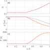 |
Figure 4. Steady-state flow fields as a function of the longitudinal length x/L for the geometric (…) and thermal throat (- - -) choking cases obtained from the CFD solver. The steady Mach number ( |


For both thermally and geometrically choked flow configurations, the steady Mach number profiles are similar, with a maximum relative deviation of approximately 5 × 10⁻⁴ between the two cases. As the velocity increases, the static pressure decreases accordingly. In the thermally choked configuration, energy addition causes the static temperature to rise from T in = 560 K at the inlet to T * ≈ 1740 K at the throat. This significant temperature increase induces a variation in the heat capacity ratio, from γ in = 1.379 to γ * = 1.304, highlighting the importance of accounting for this variation in the quasi-one-dimensional linear acoustic model ((Eq. 6)).
This steady flow-field is used to as an input to quasi-one-dimensional linear acoustic model ((Eq. 6)).
5 Discussion and results
5.1 Validation of the critical-throat acoustic-boundary condition
The GEN boundary condition (Eqs. (21) and (22)) is validated using thermally and geometrically choked flow configurations. To this end, the Euler equations are solved using both the quasi-one-dimensional linear acoustic model equation (6) and the CFD solver described in Section 4.3. To highlight the impact of the new critical-throat boundary condition, results from the quasi-one-dimensional linear acoustic model using the QSS boundary condition ((Eq. 19)) are also presented.
Figure 5 shows the normalized critical-throat Mach number fluctuations,  , resulting from the isentropic acoustic forcing defined in equation (17), plotted as a function of the dimensionless frequency
  . Both thermally choked and geometrically choked configurations are considered. Results are shown for the CFD solver: thermal throat (⃘) and geometric throat (⃣); and for the quasi-one-dimensional linear acoustic model using either the GEN or the QSS boundary conditions, respectively: thermal throat (- - -, - · -) and geometric throat (…., - … … - …).
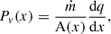
Based on the GEN boundary condition detailed in equations (21) and (22), the analytical expression for the normalised critical-throat Mach number fluctuations is given by:
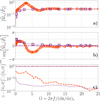 |
Figure 5. Modulus (a) and phase angle (b) of the normalized critical Mach number fluctuations due to isentropic acoustic forcing at the inlet ((Eq. 17)), |


![Mathematical equation: $$ \begin{aligned} \dfrac{\widehat{\mathrm{M} }_*}{\widehat{P}_*}&= \left[\dfrac{\bar{g}_P}{\bar{g}_U} - \bar{\gamma }_* \dfrac{\left(1+\kappa _* \bar{T}_*\right)}{2}\right] \nonumber \\&\quad + \left[\dfrac{\bar{g}_D}{\bar{g}_U} - \dfrac{\left(1+\kappa _* \bar{T}_*\right)}{2}\right] \dfrac{\widehat{D}_*}{\widehat{P}_*}\cdot \end{aligned} $$](/articles/aacus/full_html/2025/01/aacus250104/aacus250104-eq98.gif) (27)
(27)
The relative deviation between the quasi-one-dimensional linear acoustic model (L) results (with GEN or QSS boundary condition) and the CFD results is quantified as  . The forcing amplitude is set to
  , ensuring that non-linear effects remain negligible. To verify the linearity of the response, three frequencies Ω = [3, 8.5, 22] were tested with two isentropic forcing amplitudes (|P′in|=1 × 10⁻² and 1 × 10⁻³). The relative deviations between the responses were on the order of 1 × 10⁻³, confirming linear behaviour.
For the geometric-throat configuration, the QSS boundary condition  (- · · - ·) is only valid in the very low-frequency limit and is generally inaccurate. A relative error of 100% is obtained when Mach number fluctuations are imposed to vanish at the throat. In contrast, the linear model using the GEN boundary condition (….) closely matches the CFD results (⃞), with a maximum deviation of approximately 2% at very low frequencies, which decreases monotonically as the frequency increases.
In the thermally choked configuration, the GEN boundary condition also performs well, with deviations of about 10% for Ω < 7, dropping below 0.1% at higher frequencies, demonstrating the accuracy of the proposed linear acoustic model (- - -). At very low frequencies, a finite value of the normalized Mach number fluctuations  is observed in the thermal throat configuration due to the presence of the volumetric power addition P
v
, contradicting the commonly used QSS assumption (- · -). Note that applying the QSS condition, M′* = 0, leads to a local singularity in the acoustic field at the critical-throat, which contradicts the physical assumption of a continuous and smooth solution.
is observed in the thermal throat configuration due to the presence of the volumetric power addition P
v
, contradicting the commonly used QSS assumption (- · -). Note that applying the QSS condition, M′* = 0, leads to a local singularity in the acoustic field at the critical-throat, which contradicts the physical assumption of a continuous and smooth solution.
Under the GEN boundary condition, a local maximum in the deviation is observed proximate to the frequency at which the normalized critical Mach number fluctuation  peaks. This maximum, occurring at Ω = 3.1, is primarily attributed to the generation of entropy waves induced by the propagation of acoustic waves through a heated medium. For an unheated flow, i.e., in the geometric throat case, the density and pressure fluctuations satisfy
  across all frequencies, resulting in the absence of a local maximum, as shown in Figure 5. In contrast, for a heated flow, the ratio
  becomes strongly dependent on the entropy generation term,
  , since the density fluctuations
  are directly linked to entropy fluctuations via equation (11). At low frequencies (0 < Ω < 3.1), the entropy waves generated by the propagation of acoustic waves induce additional pressure fluctuations, thereby amplifying the Mach number fluctuations at the critical throat. At moderate frequencies (3.1 < Ω < 10), the generation of entropy waves induced by acoustic forcing decreases, leading to reduced Mach number fluctuations at the throat. At high frequencies, Ω = 𝒪(10), the ratio
  asymptotically approaches unity, indicating that acoustic wave propagation no longer generates significant entropy fluctuations.
Figure 6 shows the response at the critical throat under entropy-wave forcing defined by equation (18) for both geometric-throat (…., - · · - ·) and thermal-throat (- · · - ·, - · -) choking configurations. These are computed using the quasi-one-dimensional linear acoustic model with the GEN (Eqs. (21) and (22)) and QSS ((Eq. 19)) boundary conditions, respectively. The corresponding CFD results are also shown for the thermal-throat (⃘) and geometric-throat (⃞) cases. The normalized critical Mach number fluctuations,  , are plotted as a function of the dimensionless frequency
  .
.
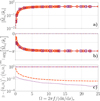 |
Figure 6. Modulus (a) and phase angle (b) of the normalized critical Mach number fluctuations, |


The relative deviation between the quasi-one-dimensional linear acoustic model (L) and the CFD simulations is quantified as  . The amplitude of the incoming entropy wave,
  , is set to the order of 10−2, ensuring that non-linear effects remain negligible. For the geometric-throat case (⃞), the deviation between CFD and the linear model with the GEN boundary condition remains within a few percent at low frequencies and decreases rapidly as frequency increases. In the thermally choked configuration (⃘), a larger deviation, up to 61%, is observed at very low frequencies, but it drops below 1% for Ω > 5. In both choking cases, the QSS boundary condition yields a constant relative deviation of 100%, due to the erroneous prescription of a vanishing critical Mach number fluctuations
  .
.
For both types of inlet forcing (acoustic and entropy), the GEN boundary condition therefore demonstrates a fair accuracy in capturing the Mach number fluctuations at the critical throat for both geometrically and thermally choked configurations.
5.2 Acoustic-reflection coefficients
Figure 7 presents the acoustic-reflection coefficient,  , defined as the ratio of the upstream- to downstream-propagating acoustic waves at the inlet, for both geometric-throat and thermal-throat configurations. Results from both the quasi-one-dimensional linear acoustic model using both GEN (Eqs. (21) and (22)) or QSS ((Eq. 19)) boundary condition (lines) and CFD solver (markers) are shown as a function of the dimensionless frequency
  .
.
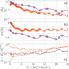 |
Figure 7. Modulus (a) and phase angle (b) of the acoustic reflection coefficient, |


For both choking configurations, a fair agreement is observed between the quasi-one-dimensional linear acoustic model using the GEN boundary condition (thermal throat: - - -, geometric throat: ….) and the CFD solver (thermal throat: ⃘, geometric throat: ⃞), as indicated by the relative deviation |1 − R a L/R a CFD|. The linear acoustic model accurately predicts the reflection coefficient for both the geometric-throat (….) and thermal-throat (- - -) configurations, with deviations remaining within 1% at low frequencies (Ω < 10) when using the GEN boundary condition. At higher frequencies (Ω > 15), however, discrepancies in both the modulus and phase angle become apparent, with deviations reaching up to 36%. This increase in deviation has been verified to be independent of the mesh resolution, time step, and forcing amplitude.
The deviation between CFD and the quasi-one-dimensional linear acoustic model using the QSS boundary condition is also shown for the geometric (- · · - ·) and thermal throat (- · -) configurations. At low frequencies (Ω < 10), the QSS boundary condition leads to deviations of up to 50% for the thermal throat case, and only a few percent for the geometric case. This highlights the importance of the GEN boundary condition in accurately capturing the behaviour of thermally choked flows, where the QSS assumption fails. For the geometric case, the improvement brought by the new boundary condition is less significant.
The entropy-noise-production coefficient,  , is plotted in Figure 8 as a function of the dimensionless frequency
  . This coefficient represents the ratio between the upstream-propagating acoustic wave
  and the incoming entropy wave
  .
.
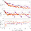 |
Figure 8. Modulus (a) and phase angle (b) of the entropy-noise production coefficient, |


Fair agreement is observed between the quasi-one-dimensional linear acoustic model using the GEN boundary condition (…. and - - -) and CFD solver (⃞. and ⃘) for both the geometric-throat and thermal-throat configurations, respectively. The relative deviation, defined as |1 − R s L/R s CFD|, remains below 2% for frequencies below Ω = 5. In all cases, the deviation remains below 25% for the thermally-choked-flow configuration (⃘) and below 8% for the geometric-throat nozzle (⃞).
The deviation between the CFD results and the quasi-one-dimensional linear acoustic model using the QSS boundary condition is higher than that obtained with the GEN boundary condition for both the thermal (- · -) and geometric (- · · - ·) throat configurations. For frequencies below Ω < 10, the QSS boundary condition results in a deviation of a few percent for the geometric case and up to 40% for the thermal throat configuration.
Here again, the linear acoustic model based on the newly proposed critical-throat boundary condition (Eqs. (21) and (22)) shows good agreement with the two-dimensional CFD results. For the thermal throat configuration, the GEN boundary condition significantly reduces the deviation between the CFD and the linear acoustic model. In contrast, the benefits of this new boundary condition are less pronounced for the geometric case.
5.3 Acoustic-transmission coefficients
The transmission coefficient is now analyzed for both geometric-throat and thermal-throat configurations. Figure 9 shows the transmission coefficient,  , as a function of the dimensionless frequency
  for both configurations, as detailed in Figure 2. Results are provided for the quasi-one-dimensional linear acoustic model using either the GEN- or the QSS-boundary conditions (lines), and for the CFD solver (markers).
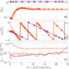 |
Figure 9. Modulus (a) and phase angle (b) of the acoustic-transmission coefficient |


The quasi-one-dimensional linear model using the GEN boundary condition (thermal throat: - - -, geometric throat: ….) accurately predicts the acoustic transmission coefficient T a , closely matching the CFD results (thermal throat: ⃘, geometric throat: ⃞) across the entire frequency range considered (Ω ≤ 25). The relative deviation, |1 − T a L/T a CFD|, quantifies the difference between the linear acoustic model and CFD solver results. For both the geometric-throat (….) and thermal-throat (- - -) configurations, the deviation remains below 2% at all frequencies.
Contrary to the behaviour observed in the geometric throat configuration, the acoustic transmission coefficient T a in the thermally choked flow remains below unity across all frequencies. This indicates that, at very low frequencies (Ω < 5), a significant portion of the acoustic wave energy is converted into entropy waves. At higher frequencies (Ω > 10), as the thermal throat approaches a purely isentropic acoustic radiation behaviour, the transmission coefficient converges toward an asymptotic value.
The deviation between the results of the CFD and the linear acoustic model using the QSS boundary condition is also detailed for both choking configurations. For the geometric case (- · · - ·), the deviation is comparable to that obtained with the GEN boundary condition, except at very low and very high frequencies, suggesting that the new boundary condition has limited benefits on the prediction of the acoustic transmission coefficient T a . In contrast, for the thermally choked case (- · - -), the QSS boundary condition induces a significant deviation, up to 140% at very low frequencies and around 10% for frequencies above Ω > 7.5. This highlights that the new boundary condition is essential for accurately predicting the acoustic behaviour in such thermally choked configurations.
Figure 10 presents the entropy-noise transmission coefficient,  , plotted as a function of the dimensionless frequency
  , for both geometric-throat and thermal-throat configurations. Results from the quasi-one-dimensional linear acoustic model (lines) and the CFD solver (markers) are shown.
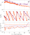 |
Figure 10. Modulus (a) and phase angle (b) of the entropy-noise-transmission coefficient |


Fair agreement is observed between the quasi-one-dimensional linear acoustic model using the GEN boundary condition (L) and the CFD solver, with deviations of only a few percent at low frequencies for both choking configurations. The deviation increases to approximately 5% at very high frequencies. In contrast, the QSS boundary condition results in more significant discrepancies: up to 5% for the geometric-throat configuration (- · · - ·), and around 22% for the thermal-throat case (- · -).
Once again, while the GEN boundary condition has a limited impact on the entropy-noise transmission coefficient T s in the geometric-throat configuration, it proves essential for accurate predictions in the thermally choked case.
6 Conclusions
Quasi-one-dimensional linear acoustic solvers are powerful tools for investigating and predicting acoustic oscillations and their sources, particularly direct and indirect combustion noise within the combustion chambers of ramjet engines. In ramjet mode, the transition from subsonic to supersonic flow is achieved through the formation of a thermal throat, driven by heat release from combustion.
In the literature, the boundary condition at the critical throat ( ) is often based on the quasi-steady assumption that Mach number fluctuations vanish, i.e., M*′=0. However, the validity of the condition is questionable, especially for thermally choked flow configurations.
In the present study, an acoustic critical-throat boundary condition applicable to both geometrically- and thermally-choked throats is proposed for non-isentropic (heated) and ideal-gas flows with a uniform composition. To validate this boundary condition, a quasi-one-dimensional linear acoustic model is developed under the same framework. Its predictions are compared against results from two-dimensional Euler flow simulations. To assess the model across a range of choking scenarios, two configurations are considered: one featuring a geometric-throat, and another exhibiting a thermal-throat induced by a steady volumetric non-uniform heat source term.
The results of the quasi-one-dimensional linear acoustic model show good agreement with those of the two-dimensional CFD simulations when the new acoustic boundary condition is applied at the critical throat. In contrast, significant deviations are observed when using the commonly adopted quasi-steady critical-throat boundary condition, M′* = 0, particularly for the transmission coefficients in the case of a thermal throat. It should also be noted that enforcing the QSS boundary condition at the critical throat introduces a local singularity in the acoustic field, which lacks physical justification. The proposed boundary condition eliminates this singularity and accurately captures the acoustic behaviour of thermally choked flow configurations, highlighting its importance for modelling such systems.
Further validation is required for additional thermally choked flow configurations, including variations in geometry and steady-state volumetric heat release profiles. To better capture the acoustic behaviour of such engines, the assumption of steady volumetric heat addition should be relaxed by explicitly modelling the thermoacoustic coupling. Finally, the single-species flow assumption will need to be lifted in order to investigate the effects of indirect compositional noise.
Conflicts of interest
The authors declare no conflicts of interest in regards to this article.
Data availability statement
The research data associated with this article are included within the article.
References
- I. Smith: The effect of dissociation in rockets, ramjets, and wind tunnels, in: Proceedings of the Institution of Mechanical Engineers, Conference Proceedings. Vol. 178. SAGE Publications, Sage UK, London, England, 1963, pp. 27–32. [Google Scholar]
- R. Fry: A century of ramjet propulsion technology evolution. Journal of Propulsion Power 20 (2004) 27–58. [Google Scholar]
- F. Falempin: Ramjet and dual mode operation, Technical Report RTP-EN-AVT-150, NATO, 2008. [Google Scholar]
- H. Wang, Q. Yang, X. Xu: Effect of thermal choking on ejection process in a rocket-based combined cycle engine. Applied Thermal Engineering 116 (2017) 197–204. [Google Scholar]
- W. Knuth, P. Gloyer, J. Goodman, R. Litchfor: Thermally-choked combustor technology, Technical 19960009786, NASA, 1993, https://ntrs.nasa.gov/citations/19960009786. [Google Scholar]
- O. Dessornes, D. Scherrer: Tests of the JAPHAR dual-mode ramjet engine. Aerospace Science and Technology 9 (2005) 211–221. [Google Scholar]
- K.-C. Lin, K. Jackson, R. Behdadnia, T. Jackson, F. Ma, V. Yang: Acoustic characterization of an ethylene-fueled scramjet combustor with a cavity flameholder. Journal of Propulsion Power 26 (2010) 1161–1170. [Google Scholar]
- F. Marble, S. Candel: Acoustic disturbance from gas non-uniformities convected through a nozzle. Journal of Sound and Vibration 55 (1977) 225–243. [Google Scholar]
- W. Moase, M. Brear, C. Manzie: The forced response of choked nozzles and supersonic diffusers. Journal of Fluid Mechanics 585 (2007) 281–304. [Google Scholar]
- I. Duran, S. Moreau: Solution of the quasi-one-dimensional linearized Euler equations using flow invariants and the Magnus expansion. Journal of Fluid Mechanics 723 (2013) 190–231. [Google Scholar]
- L. Magri: On indirect noise in multicomponent nozzle flows. Journal of Fluid Mechanics 828 (2017) R2. [Google Scholar]
- M. Huet, A. Emmanuelli, T. Le Garrec: Entropy noise modelling in 2D choked nozzle flows. Journal of Sound and Vibration 488 (2020) 115637. [Google Scholar]
- Y. Gentil, G. Daviller, S. Moreau: Combustion noise modelling of thermally perfect and multi-species gas flow in nozzles. Journal of Fluid Mechanics 1014 (2025) A39. [Google Scholar]
- F. Olivon, A. Genot, J.-E. Durand, A. Hirschberg, E. Piot: On the linear aero-acoustic response of a thermally-choked-flow nozzle to acoustic and entropy plane waves. Submitted to Journal of Sound and Vibration (2025). [Google Scholar]
- F. Olivon, A. Genot, L. Hirschberg, S. Moreau, A. Hirschberg: On the critical-throat boundary condition in quasi-one-dimensional linearised-Euler equation models. Journal of Fluid Mechanics 1019 (2025) A4. [Google Scholar]
- H.S. Tsien: The transfer functions of rocket nozzles. Journal of the American Rocket Society 22 (1952) 139–143. [Google Scholar]
- N. Karimi, M. Brear, W. Moase: Acoustic and disturbance energy analysis of a flow with heat communication. Journal of Fluid Mechanics 597 (2008) 67–89. [Google Scholar]
- S.R. Yeddula, R. Gaudron, A.S. Morgans: Acoustic absorption and generation in ducts of smoothly varying area sustaining a mean flow and a mean temperature gradient. Journal of Sound and Vibration 515 (2021) 116437. [Google Scholar]
- N. Karimi, M.J. Brear, W.H. Moase: On the interaction of sound with steady heat communicating flows. Journal of Sound and Vibration 329 (2010) 4705–4718. [Google Scholar]
- A. Giauque, M. Huet, F. Clero: Analytical analysis of indirect combustion noise in subcritical nozzles. Journal of Engineering for Gas Turbines and Power 134 (2012) 111202. [Google Scholar]
- J. Nan, J. Li, A. Morgans, L. Qin, L. Yang: Theoretical analysis of sound propagation and entropy generation across a distributed steady heat source. Journal of Sound and Vibration 536 (2022) 117170. [Google Scholar]
- V. Rani, S. Rani: WKB solutions to the quasi 1D acoustic wave equation in ducts with non-uniform cross-section and inhomogeneous mean flow properties – acoustic field and combustion instability. Journal of Sound and Vibration 436 (2018) 183–219. [Google Scholar]
- S. Basu, S.L. Rani: Generalized acoustic Helmholtz equation and its boundary conditions in a quasi 1-D duct with arbitrary mean properties and mean flow. Journal of Sound and Vibration 512 (2021) 116377. [Google Scholar]
- S. Yeddula, J. Guzmán-Iñigo, A. Morgans: A solution for the quasi-one-dimensional linearised Euler equations with heat transfer. Journal of Fluid Mechanics 936 (2022) R3. [Google Scholar]
- A. Jain, L. Magri: A physical model for indirect noise in non-isentropic nozzles: transfer functions and stability. Journal of Fluid Mechanics 935 (2022) A33. [Google Scholar]
- F. Olivon, J.-E. Durand, A. Genot, E. Piot: Unsteady forced motion of the thermal throat in a low-Mach dual-mode ramjet nozzle, in: EUCASS-3AF, 2023, p. 558. [Google Scholar]
- E. Bekaert, A. Genot, T. Le Pichon, T. Schuller: Longitudinal acoustic field in a two-phase ramjet: numerical simulation and acoustic models, in: 3rd International Conference on High-Speed Vehicle Science & Technology, 2024, p. 151. https://hal.science/hal-04616255. [Google Scholar]
- F. Olivon, J.-E. Durand, A. Genot, E. Piot: High-frequency acoustic propagation in a thermally choked low-Mach dual-mode ramjet, in: 30th AIAA/CEAS Aeroacoustics Conference (2024). American Institute of Aeronautics and Astronautics, 2024, pp. 1–15. [Google Scholar]
- J.-E. Durand, F. Olivon: Thermally choked nozzle flow 1D model for low-Mach dual mode scramjet performance assessment, in: 3rd International Conference on High-Speed Vehicle Science & Technology, 2024, p. 130. https://hal.science/hal-04948424/. [Google Scholar]
- W. Li, D. Zhao, X. Chen, Y. Sun, S. Ni, D. Guan, B. Wang: Numerical investigations on solid-fueled ramjet inlet thermodynamic properties effects on generating self-sustained combustion instability. Aerospace Science and Technology 119 (2021) 107097. [Google Scholar]
- S. Yeddula, J. Guzman Inigo, A. Morgans: Effect of steady and fluctuating heat transfer on acoustic and entropy transfer functions of a nozzle, in: 28th AIAA/CEAS Aeroacoustics (2022) Conference. American Institute of Aeronautics and Astronautics, 2022, pp. 1–12. [Google Scholar]
- Y. Gentil, G. Daviller, S. Moreau, N. Treleaven, T. Poinsot: Theoretical analysis and numerical validation of the mechanisms controlling composition noise. Journal of Sound and Vibration 585 (2024) 118463. [Google Scholar]
- E.W. Lemmon, R.T. Jacobsen, S.G. Penoncello, D.G. Friend: Thermodynamic properties of air and mixtures of nitrogen, argon, and oxygen from 60 to 2000 K at pressures to 2000 MPa. Journal of Physical and Chemical Reference Data 29 (2000) 331–385. [Google Scholar]
- E. Süli, D.F. Mayers: An Introduction to Numerical Analysis, 1 edn. Cambridge University Press, 2003. [Google Scholar]
- A.H. Shapiro: The Dynamics and Thermodynamics of Compressible Fluid Flow. Wiley, 1976. [Google Scholar]
- W. Heiser, D. Pratt: Hypersonic Airbreathing Propulsion. AIAA, Washington, DC, 1994. [Google Scholar]
- A. Refloch, B. Courbet, A. Murrone, P. Villedieu, C. Laurent, P. Gilbank, J. Troyes, L. Tessé, G. Chaineray, J. Dargaud, E. Quémerais, F. Vuillot: CEDRE software. AerospaceLab Journal (2011). https://hal.science/hal-01182463. [Google Scholar]
- C. Le Touze, A. Murrone, H. Guillard: Multislope MUSCL method for general unstructured meshes. Journal of Computational Physics 284 (2015) 389–418. [Google Scholar]
- E. Toro, M. Spruce, W. Speares: Restoration of the contact surface in the HLL-Riemann solver. Shock Waves 4 (1994) 25–34. [NASA ADS] [CrossRef] [Google Scholar]
- J. Butcher: Implicit Runge–Kutta processes. Mathematics of Computation 18 (1964) 50–64. [Google Scholar]
Appendix A
Quasi-one-dimensional critical-throat boundary condition
To obtain the quasi-one-dimensional critical-throat boundary condition model for a thermally choked flow nozzle, the quasi-one-dimensional linearized Euler equations for momentum and energy are considered using the perturbation convention  , where
  denotes the steady component and y′ the small perturbation of y = [ρ, u, p, T, c, γ]:
 (A.1)
(A.1)
where  ,
,  , and
, and  are the normalized pressure, velocity, and density fluctuations, respectively.
The steady flow velocity profile,  , is locally approximated at the throat as
  , where
  denotes the velocity gradient at the critical-throat. The origin of the coordinate
  is chosen such that the extrapolated velocity profile
  vanishes at
  . The throat position is
  . Based on this definition, the following time-space transformation is introduced as performed by Marble and Candel [8]:
The momentum and total energy equations of the linearized Euler system ((Eq. A.1)) can be rewritten using the time-space transformation as follows:
 (A.2)
(A.2)
Introducing the dimensionless frequency  , the system equation (A.2) is further expressed in the frequency domain. Applying the Fourier transform with the convention
  , the above system of equations writes:
 (A.3)
(A.3)
Subtracting the momentum equation from the energy equation yields:
 (A.4)
(A.4)
This equation is now evaluated at the steady critical-throat position. The assumption of Tsien [16], as proposed by Crocco, is used such that  ,
,  , and
, and  , as well as their derivatives, are continuous at the critical-throat location. It is further assumed that none of the derivatives are proportional to 1/(1 − ξ), as such a condition would lead to a singularity at the critical-throat.
Under these assumptions and because at the throat ξ = 1 and  , hence the term proportional to
  vanishes and the boundary condition at the critical-throat position becomes equation (21).
Appendix B
CEDRE solver
The unstructured Computational Fluid Dynamics (CFD) ONERA code CEDRE [37] solves the classical two-dimensional Euler equations:
 (B.1)
(B.1)
where ρ denotes the mass density, u = (u, v) the velocity vector, p the static pressure, e 0 = e + |u|2/2 the total specific energy (e being the specific internal energy), P v the volumetric heat source term, t the time, ∇ the Nabla operator, and ⊗ denotes the outer product.
The potential influence of computational resolution, both spatial and temporal, has been assessed by varying the computational mesh size and time step.
Four distinct computational grids and four time-step values have been tested. The mesh size Δx was varied from 0.5 mm (235 000 grid points) to 4 mm (3000 grid points), while the time step Δt ranged from 1 × 10⁻⁷ s to 5 × 10⁻⁶ s.
The results show that the pressure as well as the velocity fluctuations (so the acoustic waves) become independent of spatial resolution for mesh sizes smaller than Δx = 1 mm at a tested frequency Ω = 30. Consequently, the selected mesh size and time step, (Δx, Δt)=(1 mm, 1 × 10⁻⁶ s), corresponding to a CFL number of  (
( and
and  being respectively the inlet steady-state longitudinal velocity and speed of sound), offer the best compromise between numerical accuracy and computational cost, yielding an absolute relative error of only 1 × 10⁻³ compared to the finest refinement.
To validate the linear acoustic response of the flow, simulations were performed at the same frequency ( ) for acoustic forcing amplitudes of 1% and 0.1%. A relative difference of less than 1 × 10⁻³ was observed in the acoustic-reflection coefficient, confirming the validity of the linear acoustics assumption.
Cite this article as: Olivon F. Genot A. Durand J.-E. Hirschberg A. & Piot E. 2025. A quasi-one-dimensional critical-throat acoustic boundary condition for thermally choked dual-mode ramjet nozzles. Acta Acustica, 9, 80. https://doi.org/10.1051/aacus/2025064.
All Tables
Nozzle-inlet Mach number Min, total temperature T 0, in, and static pressure p in, corresponding to a typical flight Mach number M = 3.
All Figures
|
Figure 1. Sketch of an idealized dual-mode ramjet incorporating a thermal throat. |
| In the text | |
|
Figure 2. Sketch of the boundary condition treatment for a thermally choked flow configuration. A similar decomposition can be applied to a nozzle with a geometric throat. |
| In the text | |
|
Figure 3. Simplified two-dimensional planar sketch of a dual-mode ramjet geometry (not to scale). |
| In the text | |
|
Figure 4. Steady-state flow fields as a function of the longitudinal length x/L for the geometric (…) and thermal throat (- - -) choking cases obtained from the CFD solver. The steady Mach number ( |
| In the text | |
|
Figure 5. Modulus (a) and phase angle (b) of the normalized critical Mach number fluctuations due to isentropic acoustic forcing at the inlet ((Eq. 17)), |
| In the text | |
|
Figure 6. Modulus (a) and phase angle (b) of the normalized critical Mach number fluctuations, |
| In the text | |
|
Figure 7. Modulus (a) and phase angle (b) of the acoustic reflection coefficient, |
| In the text | |
|
Figure 8. Modulus (a) and phase angle (b) of the entropy-noise production coefficient, |
| In the text | |
|
Figure 9. Modulus (a) and phase angle (b) of the acoustic-transmission coefficient |
| In the text | |
|
Figure 10. Modulus (a) and phase angle (b) of the entropy-noise-transmission coefficient |
| In the text | |
Current usage metrics show cumulative count of Article Views (full-text article views including HTML views, PDF and ePub downloads, according to the available data) and Abstracts Views on Vision4Press platform.
Data correspond to usage on the plateform after 2015. The current usage metrics is available 48-96 hours after online publication and is updated daily on week days.
Initial download of the metrics may take a while.