| Issue |
Acta Acust.
Volume 10, 2026
Topical Issue - Spatial and binaural hearing: From neural processes to applications
|
|
|---|---|---|
| Article Number | 11 | |
| Number of page(s) | 16 | |
| DOI | https://doi.org/10.1051/aacus/2026011 | |
| Published online | 25 February 2026 | |
Scientific Article
A blind binaural real-time model for listening effort evaluated using continuous subjective listening effort rating
1
CvO University Department für Medizinische Physik und Akustik und Exzellenzcluster “Hearing4All”, 26129
Oldenburg
Germany
2
Fraunhofer Institute for Digital Media Technology, Branch of Hearing Speech and Audio Technology, 26129
Oldenburg
Germany
* Corresponding author: This email address is being protected from spambots. You need JavaScript enabled to view it.
Received:
10
June
2025
Accepted:
26
January
2026
Abstract
This study investigated real-time assessment and modeling of perceived listening effort (LE). The model consists of a binaural front-end, followed by a monaural back-end. As front-end, a novel blind real-time implementation of the binaural speech intelligibility model (BSIM) was developed, which models spatial release from masking by considering binaural unmasking and better-ear listening simultaneously. A neural network was used as back-end, which was trained on inputs and outputs of a LE prediction model based on phoneme classification called Listening Effort prediction from Acoustic Parameters (LEAP). A novel method for evaluating binaural real-time models of LE was developed, where simulated scenes with a target speaker and a noise interferer were used, which were either co-located or spatially separated. Dynamic changes were introduced to the scene by abruptly altering the signal-to-noise ratio and/or reverberation time. Participants continuously rated subjectively perceived LE using a slider interface with LE categories, while listening to the scenes via headphones. The model accurately predicted subjective LE, especially changes in signal-to-noise ratio and binaural benefits. It also predicted detrimental effects of reverberation as observed in the experiment, although the impact of reverberation was slightly overestimated. Human response times were estimated for further tweaking the model’s integration time.
Key words: Listening effort / Real-time / Spatial hearing
© The Author(s), Published by EDP Sciences, 2026
 This is an Open Access article distributed under the terms of the Creative Commons Attribution License (https://creativecommons.org/licenses/by/4.0), which permits unrestricted use, distribution, and reproduction in any medium, provided the original work is properly cited.
1 Introduction
Estimating speech intelligibility (SI) or listening effort (LE) in real-time can be valuable for several online speech processing applications. For example, a hearing aid device could utilize such estimates to choose the optimal algorithm for varying listening conditions. This study proposes a real-time model to predict LE, along with a novel experimental assessment method to capture subjectively perceived LE in dynamically changing listening conditions.
Regarding the assessment of speech perception, SI has been a subject of research for several decades, while in recent years LE emerged as another relevant speech perception measure [1, 2]. Methods of assessing LE can be divided into physiological, subjective and performance-based procedures: Common physiological procedures are electroencephalography [3, 4], pupillometry [5, 6] and skin conductance [7]. Common subjective procedures are questionnaire assessments [8, 9], ratings on a scale and categorical ratings [10, 11]. Performance-based procedures typically include a second (not necessarily auditory) task while performing a listening task, and LE is then operationalized in terms of performance measures in the secondary task [12, 13].
SI and LE are related in a sense that LE generally increases as SI decreases and vice versa. When measured with physiological markers such as peak pupil dilation (e.g., [14–16]), it is often found that LE decreases as SI gets very low, which is commonly interpreted as a motivational component, i.e., that listeners tend to give up trying to understand speech if too much effort would be required. In contrast, when subjectively perceived LE is measured with, e.g., categorical rating scales, LE typically increases monotonically with decreasing SI, until listeners give the maximum rating (e.g., “extreme effort” [11, 17]).
While subjective assessment methods generally are easier to use and set up without high level of expertise [1], they have some problems due to their subjective nature. In [18] it was shown that participant ratings of LE strongly correlated with subjectively perceived performance. They hypothesized that people substitute the rather difficult task to rate LE with the task of rating their subjective performance. Other works also show a significant correlation of subjective performance and subjective LE [14, 19], supporting this theory. The application addressed in this study is to develop a model which could eventually be used to control a hearing aid to select the best algorithm based on lowest evoked subjectively perceived listening effort. In this context, the model should predict very high LE in conditions with very low SI (rather than predicting low LE because listeners have given up), because a hearing aid in such conditions should aim to provide signal processing which has the potential to decrease LE if motivation is given. We focus on predicting LE rather than SI, because LE can provide additional information in conditions in which speech may be quite impaired by, e.g., masking noise, but still SI can be very high. Specifically, changes in LE can be observed even if SI is at ceiling [17], making LE more relevant for desired comfortable listening conditions, e.g., in case of a positive signal-to-noise ratio (SNR).
Several model approaches to predict SI and LE have been proposed. Some of them consider that listening with two ears can improve speech recognition, and that those measures are affected by the spatial configuration of sound sources and the listener. Sound coming from a lateralized position arrives earlier at the ipsilateral ear. Likewise, the signal arriving at the contralateral ear is attenuated due to the head-shadowing effect. The differences in time of arrival (or in phase) and in level caused by lateralization are referred to as interaural time differences (ITD) or interaural phase differences (IPD) and interaural level differences (ILD), respectively. The extent of those differences depends on the degree of lateralization and, in general, SI is improved and LE is reduced when speech and noise sources have different ILDs and/or ITDs [20]. Two main factors contribute to this spatial release from masking: binaural unmasking (BU) and better-ear listening (BEL). BEL occurs when ILDs cause an improvement of the SNR. BU describes an additional unmasking effect that occurs when speech and interferer differ in their ITDs (or IPDs). Note that BEL and BU can occur to different amounts in different frequency regions. While BEL can be exploited more effectively above 1.5 kHz due to greater ILD in that frequency range, BU can be exploited more effectively below 1.5 kHz due to greater ITD sensitivity in that frequency range [21].
To account for spatial effects in realistic listening scenarios, prediction models for SI and LE should therefore implement BU and/or BEL. One approach to model both effects at once has been proposed with the binaural speech intelligibility model (BSIM) [22, 23], which implemented the Equalization Cancellation (EC) model [24]. The EC model assumes that BU can be modeled by removing ILDs and ITDs of the interferer from both ear signals (Equalization) and subtracting them (Cancellation), yielding an effective SNR improvement due to destructive interference. The BSIM first applies a gammatone filterbank to each ear signal, before applying the EC [24] processing in each filterband independently. Note that due to the fact that the EC model is applied only to these bandpass-filtered signals, it has no practical relevance for the predicted masking effect whether the EC processing is implemented using time processing or phase processing. EC processing is done by determining the set of ITDs and ILDs that maximizes the SNR. Then, for each filterband out of both unprocessed ear signals and the EC-processed signal, the one yielding the highest SNR is chosen for determining SI using the speech intelligibility index (SII) [25]. Consequently, the model does not distinguish between BEL and BU, but models them in one common process.
A shortcoming of these models is that they are not applicable in real-world scenarios, since they require the use of clean source signals, which are not available to, e.g., a hearing aid. To overcome this limitation, blind models have been proposed that do not require auxiliary information and can derive their predictions based only on the signal mixture actually arriving at the ears. One notable extension to the BSIM in that regard was introduced in [26], where the binaural processing was adapted to work blindly. However, for estimating SI from the processed signals, the SII [25] was used as a back-end, which still required clean source signals. To address this shortcoming, [27] combined the blind front-end of BSIM with the blind NI-STOI [28] and investigated prediction accuracy in several binaural conditions with speech reflections. The fully blind model was able to predict those effects almost as accurately as their non-blind baseline model. The blind front-end of BSIM was also extended in [29]: the blind front-end of BSIM [26] was combined with a blind back-end called Listening Effort prediction from Acoustic Parameters (LEAP) [30–32] instead of the SII. LEAP estimates SI and subjectively perceived LE from consecutive estimated posterior probabilities of a set of known phonemes referred to as posteriorgrams. A temporal smearing of the posteriorgrams causes SI to decrease, while subjectively perceived LE increases. This could be caused by disturbances like e.g., noise or reverberation. Predicted subjectively perceived LE increases monotonically with difficulty to understand speech while no effect of giving up is modeled. That property makes the subjective model valuable for the proposed application of using such a measure in a hearing aid to select the optimal hearing aid algorithm based on the lowest induced effort. While the model framework of [29] could, in principle, predict SI and subjectively perceived LE from the binaural ear signals alone, it still runs offline and cannot be used for real-time applications, which is the target application of the present study. Therefore, the model framework is further developed, partly simplified, and implemented more efficiently in the present study, resulting in a blind and real-time capable prediction model of subjectively perceived LE as described in detail below.
The real-time model is intended to realistically predict how human LE perception changes in time-varying acoustic conditions. As far as we know, there is no established method to measure time-varying subjective LE in human listeners. One common way to measure subjective LE is to present a stimulus (e.g., a sentence) and then have the listeners rate the perceived effort on a categorical scale [11]. During the presentation of the stimulus, the acoustic scene (SNR, reverb eration, spatial source configuration, …) is usually kept constant. In the present study, we were interested in how perceived LE changes when acoustic parameters change abruptly, and how the predictions of the developed model align with these changes. To this end, a continuous LE assessment method was developed as described below.
Conceptually similar continuous psychoacoustic assessment methods were, e.g., used in the context of, e.g., perceived loudness for stimuli altering in level over the course of time [33–35]. Participants were able to continuously rate loudness by either touching a switch next to seven presented loudness categories [33, 34] or using a slider-like interface on a computer screen [35]. However, those experiments were dedicated to investigating the relationship between instantaneous loudness and overall loudness and not to evaluate continuous model predictions. One example of a real-time assessment of speech stimuli for evaluating a model was proposed in [36], where listeners continuously rated speech quality while time-varying distortions were introduced. The course of speech distortions was pre-generated and called profiles. Each participant heard the same two profiles while rating speech quality continuously using a hardware slider with five quality categories. The subjective ratings were then compared to predictions of a speech quality model with time-varying output computed for time windows shifted along the stimuli.
The present study employed a similar concept to investigate subjectively perceived LE: time-varying profiles of speech subjected to different amounts of noise and/or reverberation were created in conditions with separated and co-located sound sources. These profiles were continuously rated by listeners using a novel, touchscreen-based interface to investigate the perceptual dynamics of LE. Additionally, reaction times of participants related to sudden changes in SNR and reverberation were estimated. The subjective ratings of LE and model predictions were quantitatively compared to evaluate the model’s prediction accuracy. The analyses also allow to determine necessary integration times for real-time LE evaluations, as a first step towards model-guided hearing devices in the future.
2 Methods
2.1 Blind real-time model
The model framework of this study was conceptually the same as in [29]. A binaural front-end processed the left and right ear signals using an EC mechanism combined with BEL, similar to the BSIM version proposed in [26]. It produced a binaurally enhanced mono output signal, which was then further processed by a LEAP back-end. The model stages had to be modified and re-implemented in order to improve computational efficiency to make it applicable for real-time usage as described below.
2.1.1 Model front-end
The front-end takes key features of the BSIM version from [26] and implements them for real-time usage in a block processing scheme. An overview of the front-end model can be seen in Figure 1.
 |
Figure 1. Overview of the front-end model. Horizontal dashed lines indicate a switch between time and spectral domain. The vertical solid line indicates the frequency-dependent split of gammatone-filterbands into EC bands and BEL bands. Processing stages marked with * use the overlap-add procedure afterwards. |
The model takes the left and right ear signals as blocks of audio x t L[k] and x t R[k] as inputs. Here, t denotes time frames and k denotes samples. An overlap-add procedure with an overlap of 50% is used for the block processing. Therefore, blocks of audio are of length 2K = 1024 samples and updated by frames of length K = 512, where K is referred to as the hopsize. The model operates at a sampling frequency of 16 kHz leading to a hopsize of 32 ms and blocksize of 64 ms. The left and right ear spectra X t L/R[f] are computed using the fast Fourier transform (FFT):
![Mathematical equation: $$ \begin{aligned} X_{t}^\mathrm{L/R}[f] = \mathcal{F} \left\{ w[k] \cdot x^\mathrm{L/R}_{t}[k] \right\} . \end{aligned} $$](/articles/aacus/full_html/2026/01/aacus250074/aacus250074-eq1.gif) (1)
(1)
Here w[k] denotes a square-root Hann window of length 2K, which is required, since the same window is used again in the reconstruction phase of the processed signal using the overlap-add procedure. The index f denotes frequency bins and ℱ the FFT operation. Only half the spectrum up to the Nyquist frequency of 8 kHz is used for efficiency since real-valued signals are processed, resulting in spectra of length  . Before applying the FFT, zero padding to 4K is applied to the block of audio
 ![Mathematical equation: $ x^{\mathrm{L/R}}_{t}[k] $](/articles/aacus/full_html/2026/01/aacus250074/aacus250074-eq3.gif) to avoid circular convolution artifacts, when doing spectral filtering later.
to avoid circular convolution artifacts, when doing spectral filtering later.
A gammatone filterbank [37] is used since the auditory processing is assumed to work for auditory bandpass filters independently. Filters are applied in the spectral domain instead of time domain for efficiency to obtain the bandpass-filtered spectra ![Mathematical equation: $ Y^{\mathrm{L/R}}_{t,b}[f] $](/articles/aacus/full_html/2026/01/aacus250074/aacus250074-eq4.gif) according to:
according to:
![Mathematical equation: $$ \begin{aligned} Y^\mathrm{L/R}_{t,b}[f] = H_{b}[f] \cdot X_t^\mathrm{L/R}[f]. \end{aligned} $$](/articles/aacus/full_html/2026/01/aacus250074/aacus250074-eq5.gif) (2)
(2)
H b [f] denotes the transfer function of the gammatone filterbank from [37], which was calculated from the filter coefficients. The index b denotes auditory filters with b = 1, …, B, where B = 29 is the total number of bandpass filters.
The front-end assumes simultaneous EC processing and BEL. Filters with a center frequency below f split = 1.5 kHz are processed using the EC procedure, which are 15 filterbands in total. Conversely, filters with a center frequency above f split are processed using BEL selection, which are 14 filterbands in total.
For each EC filterband, first, the instantaneous ILD is estimated from the ear spectra ![Mathematical equation: $ Y^{\mathrm{L/R}}_{t,b}[f] $](/articles/aacus/full_html/2026/01/aacus250074/aacus250074-eq6.gif) in dB prior to equalization, as
in dB prior to equalization, as
![Mathematical equation: $$ \begin{aligned} \alpha ^\mathrm{inst}_{t,b} = 20\cdot \log _{10} \left( \sqrt{\frac{ \sum _f|Y^\mathrm{L}_{t,b}[f]|^2}{\sum _f|Y^\mathrm{R}_{t,b}[f]|^2}} \right). \end{aligned} $$](/articles/aacus/full_html/2026/01/aacus250074/aacus250074-eq7.gif) (3)
(3)
The actual ILD values α t, b used for the EC processing are computed by taking the average over nine past frames. This corresponds to a total length of 288 ms, which is the closest integer multiple of the hopsize of 32 ms to 300 ms, proposed in [38] as the binaural sluggishness of the human binaural processing. The first equalization step is then performed resulting in ILD-equalized spectra Y t, b L, eq1 [f] and Y t, b R, eq1 [f] for the left and right ear:
![Mathematical equation: $$ \begin{aligned} \begin{aligned} Y^{\mathrm{L}, \mathrm{eq}_1}_{t,b}[f]&= Y^\mathrm{L}_{t,b}[f] \cdot 10^{-\alpha _{t,b}/40},\\ Y^{\mathrm{R}, \mathrm{eq}_1}_{t,b}[f]&= Y^\mathrm{R}_{t,b}[f] \cdot 10^{+\alpha _{t,b}/40}. \end{aligned} \end{aligned} $$](/articles/aacus/full_html/2026/01/aacus250074/aacus250074-eq8.gif) (4)
(4)
Equalization is applied in a symmetric fashion, where the left ear is attenuated by half the ILD, while the right ear is amplified by half the ILD.
Then, ITDs are calculated by first estimating the instantaneous IPD for each filterband. For this, the cross power spectral density between the right and left ear ![Mathematical equation: $ {\mathrm{\Phi}}^{\mathrm{LR}}_{t,b}[f] $](/articles/aacus/full_html/2026/01/aacus250074/aacus250074-eq9.gif) is computed. The frequency bin-wise phase is retrieved by computing the angle of the cross power spectral density and performing phase unwrapping over frequency bins. Instantaneous IPDs are then computed as:
is computed. The frequency bin-wise phase is retrieved by computing the angle of the cross power spectral density and performing phase unwrapping over frequency bins. Instantaneous IPDs are then computed as:
![Mathematical equation: $$ \begin{aligned} \varphi ^\mathrm{inst}_{t,b} = \sum _f \angle \mathrm{\Phi }^\mathrm{LR}_{t,b}[f] \frac{|\mathrm{\Phi }^\mathrm{LR}_{t,b}[f]|}{\sum _f |\mathrm{\Phi }^\mathrm{LR}_{t,b}[f]|}, \end{aligned} $$](/articles/aacus/full_html/2026/01/aacus250074/aacus250074-eq10.gif) (5)
(5)
where ∠ denotes the angle operator to retrieve the bin-wise unwrapped phase.
Instantaneous ITDs are then calculated applying the following equation:
 (6)
(6)
Here f c denotes the center frequencies of each auditory filterband. Also, instantaneous ITDs are computed by taking the average over the nine frames of the past 288 ms resulting in τ t, b . The second equalization step is then performed resulting in fully equalized spectra Y t, b L, eq2 [f] and Y t, b R, eq2 [f] for the left and right ear according to
![Mathematical equation: $$ \begin{aligned} \begin{aligned} Y^{\mathrm{L}, \mathrm{eq}_2}_{t,b}[f]&= Y^{\mathrm{L}, \mathrm{eq}_1}_{t,b}[f] \cdot e^{-j \pi f \cdot \tau _{t,b}},\\ Y^{\mathrm{R}, \mathrm{eq}_2}_{t,b}[f]&= Y^{\mathrm{R}, \mathrm{eq}_1}_{t,b}[f] \cdot e^{+j \pi f \cdot \tau _{t,b}}. \end{aligned} \end{aligned} $$](/articles/aacus/full_html/2026/01/aacus250074/aacus250074-eq12.gif) (7)
(7)
ITDs are also equalized in a symmetric fashion. Finally, the cancellation step is performed. Similar to [26], two approaches are used: The first one is supposed to increase the SNR by means of destructive interference, minimizing the signal energy of an interfering source by subtracting the equalized ear signals. This is the usual way the EC model [24] is applied. The second one aims to increase the SNR by means of constructive interference, maximizing the signal energy of a target source by adding the equalized ear signals. Therefore, the signals are computed according to
![Mathematical equation: $$ \begin{aligned} \begin{aligned} Y^{\min }_{t,b}[f] = Y^{\mathrm{L}, \mathrm{eq}_2}_{t,b}[f] - Y^{\mathrm{R}, \mathrm{eq}_2}_{t,b}[f],\\ Y^{\max }_{t,b}[f] = Y^{\mathrm{L}, \mathrm{eq}_2}_{t,b}[f] + Y^{\mathrm{R}, \mathrm{eq}_2}_{t,b}[f]. \end{aligned} \end{aligned} $$](/articles/aacus/full_html/2026/01/aacus250074/aacus250074-eq13.gif) (8)
(8)
![Mathematical equation: $ Y^{\min}_{t,b}[f] $](/articles/aacus/full_html/2026/01/aacus250074/aacus250074-eq14.gif) denotes the signal obtained by using the level minimization strategy, while
denotes the signal obtained by using the level minimization strategy, while ![Mathematical equation: $ Y^{\max}_{t,b}[f] $](/articles/aacus/full_html/2026/01/aacus250074/aacus250074-eq15.gif) denotes the signal obtained by using the level maximization strategy. The effectiveness of the cancellation step in terms of improved SNR is very dependent on the accuracy of estimated ILDs and ITDs. Also, ITDs of target and interferer have to be different for the binaural processing to produce a notable SNR improvement. In order for the minimization strategy to work, estimated ILDs and ITDs have to match the actual ones of the interferer signal. Likewise, the maximization can only lead to an increase in SNR if estimated ILDs and ITDs are close to the ones of the target signal.
denotes the signal obtained by using the level maximization strategy. The effectiveness of the cancellation step in terms of improved SNR is very dependent on the accuracy of estimated ILDs and ITDs. Also, ITDs of target and interferer have to be different for the binaural processing to produce a notable SNR improvement. In order for the minimization strategy to work, estimated ILDs and ITDs have to match the actual ones of the interferer signal. Likewise, the maximization can only lead to an increase in SNR if estimated ILDs and ITDs are close to the ones of the target signal.
The decision which one of the two alternative spectra ![Mathematical equation: $ Y^{\min}_{t,b}[f] $](/articles/aacus/full_html/2026/01/aacus250074/aacus250074-eq16.gif) and
and ![Mathematical equation: $ Y^{\max}_{t,b}[f] $](/articles/aacus/full_html/2026/01/aacus250074/aacus250074-eq17.gif) is chosen is done in the selection step: Since this is also supposed to work blindly, a measure is needed to determine which EC strategy leads to the greater SNR improvement. For this, a very simple speech modulation detection approach inspired by the speech-to-reverberation modulation energy ratio (SRMR) by Falk et al. [39] is used.
is chosen is done in the selection step: Since this is also supposed to work blindly, a measure is needed to determine which EC strategy leads to the greater SNR improvement. For this, a very simple speech modulation detection approach inspired by the speech-to-reverberation modulation energy ratio (SRMR) by Falk et al. [39] is used.
Since the SRMR requires analytic signals for each gammatone filterband, the analytic time signal is calculated using the inverse FFT as:
![Mathematical equation: $$ \begin{aligned} \begin{aligned} \hat{y}_t[k] = \mathcal{F} ^{-1} \left\{ u[f] \cdot Y_t[f] \right\} , \\ \text{ with}~u[f] = {\left\{ \begin{array}{ll} 2&\text{ if} f < F \ \\ 1&\text{ if} f = F \ \\ 0&\text{ if} f > F, \end{array}\right.} \end{aligned} \end{aligned} $$](/articles/aacus/full_html/2026/01/aacus250074/aacus250074-eq18.gif) (9)
(9)
where u[f] denotes an adapted step function centered at the Nyquist frequency at frequency bin F and ![Mathematical equation: $ \hat{y}_t[k] $](/articles/aacus/full_html/2026/01/aacus250074/aacus250074-eq19.gif) denotes the analytic signal in the time domain of any spectrum Y
t
[f]. Zero-padding introduced before applying the FFT in equation (1) is reversed by cropping the length of
denotes the analytic signal in the time domain of any spectrum Y
t
[f]. Zero-padding introduced before applying the FFT in equation (1) is reversed by cropping the length of ![Mathematical equation: $ \hat{y}_t[k] $](/articles/aacus/full_html/2026/01/aacus250074/aacus250074-eq20.gif) to 2K again.
to 2K again.
Signal reconstruction is achieved by using the overlap-add method:
![Mathematical equation: $$ \begin{aligned} \hat{y}^\mathrm{ola}_{t,b}[k] = w[k] \cdot \hat{y}_{t-1, b}[k] + w[k+K] \cdot \hat{y}_{t,b}[k+K]. \end{aligned} $$](/articles/aacus/full_html/2026/01/aacus250074/aacus250074-eq21.gif) (10)
(10)
Here w[k] denotes the square-root Hann window, as used in equation (1), and  any bandpass-filtered analytic signal in time domain of length 2K.
Following the steps of the SRMR [39], the envelope of any analytic signal ![Mathematical equation: $ \hat{y}^{\mathrm{ola}}_{t,b}[k] $](/articles/aacus/full_html/2026/01/aacus250074/aacus250074-eq23.gif) is computed as the absolute value of
is computed as the absolute value of ![Mathematical equation: $ \hat{y}^{\mathrm{ola}}_{t,b}[k] $](/articles/aacus/full_html/2026/01/aacus250074/aacus250074-eq24.gif) . In [39] the envelopes were routed into a modulation filterbank of eight modulation filters, where the lowest four were assumed to represent speech and the highest four assumed to represent noise. We found this approach as too costly in terms of processing speed, which is crucial for an application in real-time. Instead, one modulation filter for detecting modulation typical for speech and one for detecting modulation typical for noise are used. Both filters were designed to roughly match the frequency range of modulation filters used in [39] to detect speech and noise modulation, respectively. Butterworth bandpass filters of first order were used with a center modulation frequency of f
m
low = 8 Hz for detecting speech modulation and f
m
high = 32 Hz for detecting noise modulation. Both filters have a bandwidth of two octaves each, resulting in a −3 dB crossover of filters at a modulation frequency of 16 Hz. The output of the modulation filters was buffered up to 8 frames, corresponding to a total length of 256 ms. This was done according to [39], to detect speech modulation at the lower end of modulation frequencies.
. In [39] the envelopes were routed into a modulation filterbank of eight modulation filters, where the lowest four were assumed to represent speech and the highest four assumed to represent noise. We found this approach as too costly in terms of processing speed, which is crucial for an application in real-time. Instead, one modulation filter for detecting modulation typical for speech and one for detecting modulation typical for noise are used. Both filters were designed to roughly match the frequency range of modulation filters used in [39] to detect speech and noise modulation, respectively. Butterworth bandpass filters of first order were used with a center modulation frequency of f
m
low = 8 Hz for detecting speech modulation and f
m
high = 32 Hz for detecting noise modulation. Both filters have a bandwidth of two octaves each, resulting in a −3 dB crossover of filters at a modulation frequency of 16 Hz. The output of the modulation filters was buffered up to 8 frames, corresponding to a total length of 256 ms. This was done according to [39], to detect speech modulation at the lower end of modulation frequencies.
The modulation energy at the low and high modulation center frequency  is calculated using
![Mathematical equation: $$ \begin{aligned} \epsilon ^{\mathrm{low}/\mathrm{high}}_{t,b} = \sum _{k}^{\kappa }z^{\mathrm{low}/\mathrm{high}}_{t,b}[k]^2, \end{aligned} $$](/articles/aacus/full_html/2026/01/aacus250074/aacus250074-eq26.gif) (11)
(11)
where ![Mathematical equation: $ z^{\mathrm{low}/\mathrm{high}}_{t,b}[k] $](/articles/aacus/full_html/2026/01/aacus250074/aacus250074-eq27.gif) represents the buffered modulation filter output, which is of length κ = 8K and is updated for every frame. Note that in contrast to [39], where whole signals were processed offline, here, no averaging of modulation energy over time frames was performed. Additionally, since an estimate of the modulation energy is required for each gammatone filterband, no averaging of energy is performed over gammatone filterbands.
represents the buffered modulation filter output, which is of length κ = 8K and is updated for every frame. Note that in contrast to [39], where whole signals were processed offline, here, no averaging of modulation energy over time frames was performed. Additionally, since an estimate of the modulation energy is required for each gammatone filterband, no averaging of energy is performed over gammatone filterbands.
Finally, the ratio of speech-to-noise modulation energy R is calculated:
 (12)
(12)
The selection whether to use the minimization or maximization strategy is done by checking which out of the signals ![Mathematical equation: $ \hat{y}^{\min}_{t,b}[k] $](/articles/aacus/full_html/2026/01/aacus250074/aacus250074-eq29.gif) and
and ![Mathematical equation: $ \hat{y}^{\max}_{t,b}[k] $](/articles/aacus/full_html/2026/01/aacus250074/aacus250074-eq30.gif) yields a higher ratio for each EC filterband.
yields a higher ratio for each EC filterband.
Similarly, BEL is implemented for each BEL filterband by checking which out of the two ear signals ![Mathematical equation: $ \hat{y}^{\mathrm{L}}_{t,b}[k] $](/articles/aacus/full_html/2026/01/aacus250074/aacus250074-eq31.gif) and
and ![Mathematical equation: $ \hat{y}^{\mathrm{R}}_{t,b}[k] $](/articles/aacus/full_html/2026/01/aacus250074/aacus250074-eq32.gif) yields a higher ratio. Selected filterband signals are added again using overlap-add according to equation (10) for blending consecutive selected frames using a Hann window. Finally, the real parts of selected bands
yields a higher ratio. Selected filterband signals are added again using overlap-add according to equation (10) for blending consecutive selected frames using a Hann window. Finally, the real parts of selected bands ![Mathematical equation: $ \hat{y}_{t,b}^{\mathrm{sel}}[k] $](/articles/aacus/full_html/2026/01/aacus250074/aacus250074-eq33.gif) are added up to one final output signal
are added up to one final output signal ![Mathematical equation: $ y^{\mathrm{out}}_{t,b}[k] $](/articles/aacus/full_html/2026/01/aacus250074/aacus250074-eq34.gif) , which is the output of the front-end model:
, which is the output of the front-end model:
![Mathematical equation: $$ \begin{aligned} y_t^\mathrm{out}[k] = \sum _b^B \mathfrak{Re} \left\{ \hat{y}_{t,b}^\mathrm{sel}[k] \right\} . \end{aligned} $$](/articles/aacus/full_html/2026/01/aacus250074/aacus250074-eq35.gif) (13)
(13)
2.1.2 Model back-end
A version of LEAP trained using a teacher-student approach serves as the back-end. The teacher-student approach describes a procedure in which a student model is trained on the inputs and outputs of a pre-trained teacher model. The student model had been developed prior to this study for real-time usage in German TV and broadcasting, for which its latency and computational efficiency had to be reduced. This way, the time-consuming operations of LEAP are avoided whilst retaining most of its estimation performance. The neural network architecture shown in Figure 2 was used. It is based on QuartzNet [40] and primarily consists of one-dimensional convolutions (1D-Conv). At the input layer, mel-spectrograms of M = 35 time frames and N = 100 frequency bins are fed into the model. They are then processed by a 1D-Conv layer with a kernel size of 3 along the time dimension and a rectified linear unit (ReLU) for activation. Zero padding is used to keep the data shape constant.
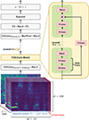 |
Figure 2. Neural network structure of the student version of LEAP. |
The main processing stage consists of time-channel separable convolutions (TCS-Conv), also known as depthwise separable convolution, which are based on 1D-Conv operations that utilize the channel dimension in order to process two-dimensional data. TCS-Conv comprise a depthwise convolution (D-Conv) and a pointwise convolution (P-Conv). First, a D-Conv is applied where for each of the N channels (frequency bins) separate kernels that span across all M time frames are used. For P-Conv, a single kernel of size 1 that spans across all N channels yields outputs for each individual time frame. All input and output channels share a weighted connection with a total of N 2 weight parameters, for a constant number of channels. A single TCS-Conv, as used in this work, requires M N + N 2 + 2N model parameters.
In the main processing stage, five blocks, each containing five TCS-Convs with ReLU activation, are applied. The data shape is retained at N × M by using zero padding and keeping the number of channels constant for all Conv operations. An additive skip connection spans from the beginning to the end of each block and contains an extra P-Conv layer.
After these TCS-Conv blocks, feature data are processed by means of a 1D-Conv layer with kernel size 3 without zero padding. Max pooling is applied such that the time dimension is reduced to a single frame, resulting in a vector of length N. Next, two fully connected layers with intermediate ReLU activation reduce the channel dimension to a single frequency bin, leaving a single scalar value as their output. The output is then scaled to a value between 0 and 1 with a sigmoid function. Mapping this value o with
 (14)
(14)
yields the final estimation of listening effort  between 1 and 13 effort scale categorical units (ESCU), as used for the German dataset in [32]. While for the hypothetical application of this study to use the model on a hearing aid to choose the best algorithm in terms of the lowest LE value, it might not be entirely necessary to scale the back-end output to the ESCU-range, we still apply this mapping to be in line with previous works [10, 11, 31] and make the output interpretable. Overall, the neural network comprises 458 301 trainable model parameters.
The model was trained on mixture signals of German speech and noise. Training and validation sets were generated in the same way, but with different, non-overlapping splits of the employed data corpora, as shown in Table 1.
Non-overlapping splits in training and validation of the employed data corpora for speech and noise.
Speech data were taken from the German version of CommonVoice 7.0 [41]. A crowdsourcing-based corpus, it mainly contains recordings by non-professional speakers made on their consumer devices. With a total of 1035 h of German speech recorded by 15 620 speakers, it provides a large dataset as well as a wide variety of speakers and sound quality. Since only 8% of the data were recorded by female speakers, most of the utterances recorded by males were discarded in order to achieve a balanced representation of both genders. The data with validated transcripts were used for the training set, those with unvalidated transcripts for the validation set. Speechocean King-ASR-187 [42], a corpus containing about 100 h of German speech data, was additionally used for the training set. The combined speech data of both corpora were used a total of three times to reach around 1000 h of speech data. Noise data were taken from several different corpora: BBC Sound FX [43] contains a variety of noise types, ranging from human-made sounds to engine noises. MUSAN [45] comprises 929 noise recordings and more than 42 h of music of different genres. The speech data of MUSAN were not used in this work, since the amount of German speech data is negligible compared to the CommonVoice and Speechocean corpora. 997 noise recordings from the corpus provided as part of the Deep Noise Suppression (DNS) Challenge [44] were also used. Training data were built using all the noise data from the BBC and DNS corpora, as well as 2/3 of the music of MUSAN. These noise signals were assumed to provide enough variety in order to create degraded speech signals that elicit a wide range of listening effort scores, when mixed with speech at different SNRs. The remaining 1/3 of MUSAN’s music as well as all of its noise data were used for the validation set, allowing it to be small, yet diverse.
Pairs of speech and noise signals were randomly selected and the noise adjusted to match the speech signal’s length. This was done by truncation if the noise signal was longer than the speech signal or by repetition if it was shorter. Speech and noise were added at a random SNR of −10, −6, −2, 2, 6, 10, 14, 18, or 22 dB. SNRs were applied using the active speech level according to ITU P.56 [46]. 28% of the total data were clean speech without any noise. 95% of the data were convolved with one of 60k simulated room impulse responses (RIR), originating from the corpus of [47].
In order to make the model more robust against other disturbances occurring in TV and broadcasting besides noise, the training set was extended with a subset of low-resolution MP3-encoded speech. MP3 encoding occurred at 8, 16, 24, 32, 48 and 56 kilobits per second. Half of the subset’s speech signals were bandpass-filtered between 300 Hz and 3.4 kHz using a second-order Butterworth filter in order to simulate speech transmitted via telephone. Half of the subset’s data were convolved with a simulated RIR, and only 48% were mixed with noise at 2, 6, 10, 14, 18 or 22 dB SNR. In total, the training and validation sets contained around 1026 h and 7:39 h of audio, respectively.
Data were fed to the model as mel-spectrograms with non-overlapping frames of 30 ms length and 100 frequency bins. In order to produce more reliable estimates during real-time usage, each time frame is provided with temporal context. Besides the current time frame for which the estimation is being made, the 33 preceding frames (0.99 s) and the following frame are additionally given. By using a future time frame, the system has an algorithmic latency of at least two frame lengths (60 ms). Training took place with a batch size of J = 400 signal frames and lasted for 28 epochs. The mean squared error
 (15)
(15)
was used as the loss function, with  being the estimated LE scores for the j-th signal frame within a batch. The label l
j
is the desired estimate for the j-th signal frame obtained from the output of the original LEAP model. Model parameters were optimized using ADAM [48] with an initial learning rate of 10−4.
being the estimated LE scores for the j-th signal frame within a batch. The label l
j
is the desired estimate for the j-th signal frame obtained from the output of the original LEAP model. Model parameters were optimized using ADAM [48] with an initial learning rate of 10−4.
To calculate the speed-up factor, the proposed back-end and original LEAP were run on 1000 consecutive frames and processing time averaged per frame. The student version of LEAP required 1.45 ms to process one frame compared to 3.70 ms for LEAP, which implies a speed-up factor of about 2.55 for the proposed back-end.
2.2 Real-time subjective evaluations
A novel measurement method was developed to assess subjective continuous LE in human participants for dynamic acoustic scenes to evaluate the model output. Similarly to the work presented in [36], time-continuous profiles were used. In the current work, profiles only contained abrupt changes and were applied to parameters of a simulated binaural scene. The simulation was done using the toolbox for acoustic scene creation and rendering (TASCAR) [49], which implements higher-order Ambisonics.
The acoustic scene is depicted in Figure 3. It consisted of one target speaker and one noise interferer with a distance of 10 m to the receiver. The receiver was placed asymmetrically inside a 30×16×9.1 m3 room to allow for multiple reflection paths of different lengths. Two spatial conditions were simulated in order to control the effect of binaural unmasking. Both sources were either placed in front of the receiver (S0N0) or rotated around the receiver by 45° in opposite directions (S−45N+45). A general head-related transfer function from TASCAR was used. RIRs were rendered from the scene, so that stimuli could be generated by convolving speech and noise with their respective RIRs.
 |
Figure 3. Sketch of the simulated room using TASCAR with dimensions 30×16×9.1 m3. The receiver was displaced from the middle of the room by −5 m in x direction and −3 m in y-direction and located 1.8 m above ground, while rotated by 22° counter-clockwise. Sound sources were located 10 m in front of the receiver in the frontal condition S0N0 or rotated around the receiver by 45° in opposite directions in the lateralized condition S−45N+45. |
The German tale “Zwerg Nase” [50] (engl. “Dwarf Nose”) was used as speech material, which had been used prior to this study in [51], in which speech pauses were cut to a maximum of 500 ms. The tale was further adapted by splitting the tale into segments of five minutes each, which will be further referred to as chapters. For each chapter, a questionnaire was developed consisting each of four questions with four answer options each plus an option “I don’t know”. As interferer, ICRA1 noise was used, which is a continuous and nearly unmodulated noise spectrally shaped to correspond to a male talker [52]. While the model back-end was trained with different types of interferers, like everyday noise or music, the back-end is able to generalize for ICRA1 noise as observed in early experiments. No further noise types, such as used in the training, were used to keep the duration of the hearing experiment described here short. A final stimulus consisted of one chapter each, where different profiles were applied as described in the following.
Each profile of 300 s length included 30 parameter changes. Those parts, where the modified parameter stayed constant, are further referred to as sections. One third of all section lengths was set to each of 7, 10, and 13 s, respectively, and the order of occurrence was randomized to avoid overly predictable time points at which acoustic changes occurred.
As scene parameters, SNR and reverberation time T 60 were chosen, where T 60 describes the duration in seconds for the diffuse level to drop by 60 dB after a source stops emitting sound. Diffuse reverberation was achieved by using TASCAR’s implementation of a feedback delay network, which takes T 60 as input. Early reflections were rendered up to two consecutive wall reflections using image source models. In order to observe single and combined effects, they were either adapted while the other parameter stayed constant or parameters were adapted simultaneously. This led to three distinct profiles: SNR only, T60 only and SNR+T60. For the SNR only profile, only additive noise was added without any reverberation. For the T60 only profile, no noise was added and speech was reverberated with RIRs of different T60 values. Four seconds of audio before the actual section were used when convolving with RIRs and discarded afterwards, if reverberation was applied. That way, reverberation was approximately fully built up in the section of interest. For the SNR+T60 profile, both noise and reverberation were used. While the temporal sequence of SNRs and T60 values was randomized differently for the three profiles, the exact same temporal pattern was used within each profile for the S0N0 and the S−45N+45 conditions. The two spatial setups thus differed only in the spatial source configuration, while all other parameters and their temporal changes were the same. This was done to be able to analyze the role of the binaural benefit independently from temporal parameter changes. Additionally, a training profile was used, where for every section one of the six profiles was selected at random and parameters adapted the respective way. In this case, the tale “Der Jäger und der Zwergenprinz” [53] (engl. “The hunter and the dwarven prince”) spoken by a different male talker was used, where the same modifications as for the other tale were applied by Mirkovic et al. [51].
When generating profiles, parameters were drawn at random from uniform distributions, which can be seen in Table 2. The direct-to-reverberant ratios for the used reverberation times T60 for all generated RIRs can be seen in the supplementary material in Section S1.
Distributions used for generating each profile. Ranges are displayed as start : step size : end. Note that gains marked with * indicate actual gain increases to the speech signal relative to 65 dB SPL, while for the other profiles it symbolizes a change in SNR relative to 65 dB SPL. SNR is applied by amplifying speech by half of the SNR and by attenuating noise by half of the SNR. A T60 of 0 s indicates an anechoic setting. The time courses of the parameter changes over time are also displayed in the results sections.
Changes of SNR were applied by amplifying speech by half of the SNR and attenuating noise by half of the SNR. That way, the overall level was reduced compared to applying the SNR to one signal type only, preventing a biased perceived subjective LE due to high loudness and producing uncomfortably high sound pressure levels. An SNR of 0 dB corresponded to a speech and noise level of 65 dB SPL each. SNRs were applied before convolving with RIRs and slight changes in level due to intrinsic level variations were not accounted for. High T 60 values were chosen to achieve reverberation that was considered effortful in pilot experiments. Furthermore, random overall level roving between −3 and 3 dB (step size 1 dB) was applied to each section to avoid a bias of perceived subjective LE due to constant loudness of stimuli.
This procedure produced six fixed 300 s long profiles of temporal changes in SNR and/or T 60 that were used for each participant. In order to minimize systematic training effects, the six profiles were assigned to each participant in random order. However, since the chapters of the story used as speech material needed to be presented in chronological order for the tale to make sense, the chapters were always presented in the same order. This meant that each participant listened to different combinations of speech and profiles. The only exception was the training stimulus, which consisted of the same speech stimulus combined with the training profile.
For gathering real-time feedback from participants, an application was developed, allowing participants to continuously assess perceived subjective LE using a slider interface that was accessible via network using a smartphone. The slider covered a range of 1 to 14 ESCU in accordance with [11]. Values were not visible but 6 categories ranging from “effortless” (1 ESCU) to “extreme effort” (13 ESCU) were displayed plus an additional category “noise only” (14 ESCU) for cases, where speech was not audible. As additional visual feedback the background color of the slider interface changed depending on the slider position ranging from green (1 ESCU) to red (14 ESCU) on the HSV color scale by Smith [54]. A Dell Latitude 5431 Notebook connected to an RME Babyface sound card with Sennheiser HD650 headphones was used. As smartphone, a Sharp Aquos D10 was provided. A network was accessed using a Fritzbox 7490 router. The measurement was conducted in a soundproof booth. The equipment was calibrated using Brüel & Kjær hardware including a Type 4153 artificial ear, a Type 2669 preamplifier and a Type 2610 measuring amplifier calibrated with a Type 4231 sound calibrator.
Thirteen female and seven male participants with a mean age of 27.7 years and standard deviation of 5.5 years took part in this study. They had normal audiometric thresholds (PTA4 < 20dB HL), were self-proclaimed German native speakers and had no red-green color blindness, which would have interfered with the changing background color of the slider app. Only three participants reported to ever have taken part in an experiment where LE was assessed. Participants received an instruction sheet, which can be seen in the supplementary material in Section S2. The sheet stated that no questions were intended during the measurement unless they concerned technical issues to avoid reproducibility issues. Participants did not take any breaks during the measurement although allowed by the instruction sheet. Before each chapter, they were asked to press a play button when they were ready. After each chapter, they were asked to turn over the corresponding questionnaire sheet regarding the contents of the just played chapter to assess if participants were still attentive. They had to correctly answer at least 50% of the questions so as not to be excluded post-measurement. This threshold was chosen to confirm that participants performed the task of listening to the tale as their main priority, while prior pilot experiments confirmed that the questionnaires were solvable. This led to the exclusion of one male participant, so that 19 participants in total were eligible to be analyzed. The questionnaire scores can be seen in the supplementary material in Section S3.
3 Results
3.1 Temporal patterns
The time courses of assessed subjective LE in ESCU plotted as median over participants with interquartile range (IQR) alongside model predictions are shown in Figures 4–6. In each figure, from top to bottom the course of LE for S0N0 is shown, then LE for S−45N+45 and lastly the presented profile. The median LE and IQR for model predictions were calculated over the combinations of each profile and the six chapters. Figure 4 shows the time courses for the SNR only profile.
 |
Figure 4. Median subjective (blue) and predicted (gray) LE time courses in ESCU for S0N0 (top panel) and S−45N+45 (middle panel) and the presented SNR only profile (bottom panel). LE is displayed with IQR displayed as a patch. |
 |
Figure 5. Median subjective (blue) and predicted (gray) LE time courses in ESCU for S0 (top panel) and S−45 (middle panel) and the presented T60 only profile (bottom panel). LE is displayed with IQR displayed as a patch. |
 |
Figure 6. Median subjective (blue) and predicted (gray) LE time courses in ESCU for S0N0 (top panel) and S−45N+45 (middle panel) and the presented SNR+T60 profile (bottom panel). LE is displayed with IQR displayed as a patch. |
Subjective LE ratings varied strongly over time, with median LE values ranging from below 3 ESCU (“very little effort”) to 13 ESCU (“extreme effort”). Within each section (see section transitions in bottom panel), LE ratings were rather stable, suggesting that listeners did not re-adjust their slider position a lot after having adapted to a change in SNR. As expected, changes in SNR caused changes in LE rating in a contrary manner (note that the SNR scale is inverted). There appeared to be a systematic delay in the response of the LE ratings after each section transition, which is analyzed further below. The subjective LE was often lower in the S−45N+45 condition by up to 3 ESCU compared to the S0N0 condition. The spatial benefit is also analyzed in more detail below. Predicted LE values followed a similar pattern with strong changes of predicted LE at section boundaries. Within each section, predicted LE varied more than the subjective median ratings. LE predictions closely matched median ratings for intermediate LE, and slightly over- and underestimated median ratings by about 1–2 ESCU at low and high LE, respectively. In other words, the model tended to avoid predicting extremely low and high ESCU values.
For the T60 only profile (Fig. 5) the course of subjectively perceived and predicted LE followed the course of the T60 parameter. In contrast to the SNR only profile, the range of LE was reduced, where most of the time the upper limit was at 9 ESCU. Also, the lateralization of the speech source did not lead to obvious differences in LE. However, the predicted LE always exceeded subjective LE throughout the stimulus in a range of 1–4 ESCU.
Figure 6 shows the results for the SNR+T60 profile. Here, the relationship between both parameters and subjective as well as predicted LE was more complicated. In the most extreme cases, high SNR in combination with low T60 led to the lowest subjective and predicted LE, respectively. This can be seen for example at 50 s, where an SNR of 6 dB and a T60 of 0 s were used. Conversely, low SNR in combination with high T60 led to the highest subjective and predicted LE, respectively. This can be seen for example around 130 s, where an SNR of −12 dB and a T60 of 5 s were used. The model again overestimated LE for sections with decreased SNR and increased reverberation, which can be seen for instance around 100 s and 200 s.
3.2 Steady-state responses
The temporal courses of LE ratings suggested that listeners required some time to converge towards a position on the slider after each section change, and that they did not strongly re-adjust their ratings until the next section change. In other words, the median ratings at the end of each section should reflect the listeners’ steady-state responses and should be comparable to ratings one would obtain in classic, non-real-time assessments where listeners rate LE after they heard the stimuli. To obtain a stable LE value for each section, a temporal mean was calculated over the last 2 s for each section for all participants and the model. This value of 2 s was determined experimentally, since low variance of LE was observed in the last 2 s. Afterwards, a median over all participants and model predictions was calculated for each section. Additionally, a linear regression analysis was performed for each profile as well as all profiles combined using an ordinary least squares model. A scatterplot displaying the relationship between predicted and subjective LE is shown in Figure 7. Here, the median of predicted LE is compared against the median of subjective LE in ESCU for each section and all profiles. The shape and color of each data point indicate the underlying profile. The results of the linear regression analysis are shown in the top left corner, including the slope, bias, squared Pearson correlation coefficient r2, intraclass correlation coefficient (ICC) for agreement, root mean square error (RMSE) and mean squared error of the residuals (MSER).
 |
Figure 7. Median of predicted LE plotted against the median of subjective LE in ESCU for each section. Different symbols represent the six different profiles. The black solid line represents the linear regression line, while the black dashed line represents the identity line. The results of the linear regression and correlation analysis are displayed in the top left corner. |
The results of the linear regression analysis for each individual profile can be seen in Table 3. For the profiles adapting only one parameter, a high coefficient of determination r2 above 0.9 could be observed except for the SNR only in S−45N+45, for which r2 was at 0.83. For the SNR+T60 profiles in S0N0 and S−45N+45, r2 values amounted to 0.84 and 0.81, respectively. In contrast, ICC values were high for SNR only, moderately high for SNR+T60 and lowest for T60 only, regardless of spatial configuration. The slope of the linear regression line was far below 1.0 except for the condition T60 only in S0, while the bias across profiles varied in a range of 1.9–4.6 ESCU. For both T60 only conditions, RMSE values were higher compared to the other profiles, exceeding 2 ESCU. While the MSER for all profiles combined was at 1.0 ESCU, it was notably lower for individual profiles. The relationship of LE depending on SNR is illustrated in the supplementary material in Section S4.
Results of a linear regression analysis performed on subjective and predicted LE for each profile as well as all profiles combined. Columns show values for the slope and bias of the regression line, r 2, ICC, RMSE and MSER.
3.3 Binaural benefit
To analyze the binaural benefit, the same steady-state LE values calculated above were used. For each participant and section ending, subjective LE values for lateralized sources were subtracted from subjective LE values for sources coming from the front. The same was done for the model predictions. The results grouped by SNR and T60 are displayed as violin plots in Figure 8. IQRs are shown as boxes, where the white line displays the median and whiskers are added as lines. Note that only data from the profiles adapting single parameters are shown, since for SNR+T60 not all possible combinations of SNR and T60 values were used. For each SNR and T60-value, a one-sided Wilcoxon test was conducted to test if ΔLE was significantly larger than 0 ESCU (i.e., if the lateralization caused a significant reduction in LE). Significance levels were corrected for multiple comparisons. In case of the SNR being adapted, the median binaural LE benefit for participants and the model decreased with increasing SNR. For the lowest presented SNR of −12 dB, median values for participants and the model amounted to 2.5 ESCU, respectively. The median LE benefit dropped to 0 ESCU for participants as well as for the model at the highest SNR. The binaural benefit was significant in the data at a significance level of at least down to α = 0.01 up to an SNR of 3 dB.
 |
Figure 8. Spatial release ΔLE for participants (blue) and the model (gray) due to lateralization of sound sources for the SNR only (upper panel) and T60 only (lower panel) profiles visualized as violin plots with box plots. Distributions are grouped by SNR and T60 values, respectively. Underlying data points are plotted as dots inside the violin shapes. Black boxes display IQRs, where the median is indicated as a white line inside. Whiskers are added as black lines. Note that for the T60 only profile and a T60 of 0 s no box and whiskers were drawn since most data points are at 0 ESCU. Significant release of LE in the subjective data is indicated with *, ** and *** for significancy levels of α = 0.05, α = 0.01 and α = 0.001, respectively. |
In case of the speech source being lateralized to −45° for the T60 only profile, the median LE release was at around 0 ESCU for participants regardless of presented T60. No significant release was observed in the data.
In contrast to that, the median predicted LE release by the model amounted to about −1 ESCU, indicating that lateralization induced a higher LE. However, with increasing T60, the predicted spatial release of LE increased to about 1 ESCU for a T60 of 5 s. Scatterplots of predicted vs. measured LE release are shown in the supplementary material in Section S5.
3.4 Response times to abrupt changes
The cross-correlation between each participant’s time-varying LE assessments and profiles was calculated for each of the six profiles to estimate the response times of participants similar to [36]. The point in time of each cross-correlation peak was determined to obtain the delay of participants.
The results can be seen as violin plots in Figure 9. Median response times were determined in a range from 1.54 to 2.16 s, while overall response times appeared to be greatest for the SNR+T60 profile and lowest for the T60 only profiles by a slight margin compared to the response times for the SNR only profiles. A Shapiro-Wilk test revealed that not all distributions were normally distributed. Therefore, a Kruskal-Wallis test was applied, which returned that at least one distribution differed significantly from one other distribution (H = 23.47, p < 0.001). Post-hoc Dunn’s tests with Bonferroni correction revealed that in S0N0 the greater response times for the SNR+T60 profile differed significantly from the lower ones for the T60 only profile at a significance level of α = 0.05. The greater response times for the SNR+T60 profile in S−45N+45 differed significantly at a level of α = 0.01 from the lower ones for the T60 only profile regardless of spatial configuration.
 |
Figure 9. Distribution of estimated response times in seconds for all six profiles displayed as violin plots. Underlying data points are plotted as dots inside the violin shapes. Significant differences between distributions are indicated with * and ** for Bonferroni corrected significancy levels of α = 0.05 and α = 0.01, respectively. |
4 Discussion
The time courses in Figures 4–6 indicate that predicted LE is in line with subjective LE. This is supported by the high r2 values and fairly low MSER values shown in Table 3. While RMSE values were fairly high, the low MSER suggest that estimation errors of the model could be made up for by applying a correction function derived from the linear regression analysis. The main discrepancy was that the model overestimated LE in the presence of reverberation, which is reflected by the comparably lowest ICC values among profile types. Judging by the ICC, predicted LE was most accurate if SNR changes only were applied and degraded with added T60 adaptions. While r2 values were somewhat comparable for SNR only and T60 only profiles, the ICC was far lower for the T60 only profiles, because it takes the total estimation error, reflected by high RMSE values, into consideration. In case of both parameters being adapted, ICC values ended up in-between the values observed for SNR only and T60 only profiles. These findings suggest that an increasing influence of T60 leads to a decrease in prediction accuracy of the model.
To investigate if the proposed back-end contributed to the overestimation of subjective LE in the presence of reverberation, the correlation analysis with the steady-state values was re-done using the original LEAP version as a back-end. The results can be seen in the supplementary material in Section S6. It was found that subjective LE was also overestimated to a similar extent when using the original LEAP. This finding suggests that the overestimation was not the cause of e.g., a faulty training routine for the student model, but rather inherited from the original teacher model. These findings could further be expanded on by investigating other room types. This could include asymmetric configurations, where wall reflections play a more prominent role rather than diffuse reverberation. Here, the binaural processing in humans and the model could be disturbed.
Apart from the model’s weakness to overestimate the effect of reverberation, the low slope values combined with a positive bias suggest that the model tends to avoid outputting extremely low and extremely high ESCU values. This can also be seen in the time courses in Figures 4–6 for very favorable or very adverse conditions, for which predicted LE is not as low or as high as responded by participants. For high LE, this can be partially explained by the fact that participants were able to rate LE on a scale of up to 14 ESCU, while the model was trained on a scale of up to only 13 ESCU. However, as can be seen in the time courses to 6, the median subjective LE does very rarely exceed values of 13 ESCU. This behavior was also seen for the teacher LEAP, as can be seen in the supplementary material in Section S6. This finding suggests that this behavior of not outputting very extreme values was learned by the student version.
As shown in Figure 8, the separation of speech and noise for the SNR only profile led to a binaural benefit in subjective LE as well as predicted LE, which increases with decreasing SNR. The release of LE in the data was significant up to an SNR of 3 dB. The data for participants for the T60 only profile, where only one speech source was presented, support this interpretation, since only diffuse reverberation was present. Surprisingly, here the model predicts increased LE by about 1 ESCU in the anechoic setting if the speech source is lateralized. Furthermore, a very subtle binaural benefit of about 1 ESCU is predicted for high reverberation. It is possible that in very favorable situations with no reverberation the processing of the front-end produces artifacts for lateralized sources that cause a slight increase in LE. In contrast, with high reverberation the front-end might be able to enhance lateralized speech over diffuse reverberation by applying the maximization approach via constructive interference, thus decreasing LE. However, this might not be the case for human processing.
When comparing the results for subjective and predicted LE to the findings from [29], the overall binaural benefit in ESCU appears to be smaller. They observed subjective LE ratings for speech in noise using an American matrix sentence test [55]. Subjective LE ratings were tracked for static SNR values ranging from −25 to +10 dB for different spatial settings. Here, the speech source was located in front of the receiver and the noise source was moved to different positions, which differs from the procedure in this work. The S0N100 condition in [29] is the closest to the S−45N+45 in this study judging by the angular distance between the speech and noise sources. Comparing the difference in LE for the S0N100 and S0N0 conditions in [29] yields a binaural benefit of about 6 ESCU at an SNR of −10 dB. This is a huge difference to the binaural benefit of 2.5 ESCU at an even smaller SNR of −12 dB in this study. One explanation could be that in [29] a closed matrix sentence test was used, which has a far higher word predictability compared to the tale used in this study. It was shown in studies investigating the SI increase when using fluctuating noise [56] or glimpsed speech [57] that the benefit was greater for closed-set speech material compared to open-set speech material. Similarly, the greater binaural benefit observed in [29] in terms of decreased LE could have been caused by the nature of the speech material.
The response times for judging LE appeared to be a little higher when SNR and T60 were adapted simultaneously, while the average response time was just below 2 s. Compared to the findings of continuous speech quality in [36], where response times around 1 s were observed, this is a large difference. A comparable response time was only achieved by very few participants (Fig. 9). Nevertheless, there are some notable differences between [36] and the procedure described here. A simple explanation could be that speech quality degradation caused by signal distortion is faster to rate than induced LE due to changes in SNR and T60. In some cases, parameter changes could have had a very little effect, so that participants reacted slower. This can be seen for example for SNR changes of just 3 dB in Figure 4 or for changes in T60 of 3 s and of 5 s in Figure 5. Another reason for the difference in response times could have been caused by the different groups of participants. In [36] participants were recruited from the lab and thus probably had experience with speech quality measurements or comparable experiments. Therefore, it might have been easier for them to rate speech quality. Participants recruited in this study had mostly not taken part in any hearing experiment revolving around LE, which is why they might have had to come up with an idea, how to rate LE over the course of the experiment. Another factor might have been the use of abrupt parameter changes only, while in [36] gradual parameter changes were observed as well. While the occurrence of an abrupt change in this study was unpredictable, gradual changes could be easier to follow once the onset of such a parameter change is noticed. This could have lowered the average response times estimated by calculating the cross-correlation of subjective LE courses and the profiles. Lastly, the overall mental load throughout the experiment from this study could have been higher, since participants had to also pay attention to the story contents and stimuli of 5 min were considerably longer than the 40 s stimuli from [36].
The novel assessment method for subjectively perceived LE introduced here produced data that reliably followed the course of the different profiles with fairly low variance. An increase of SNR led to decreased subjective LE, while an increase of T 60 led to increased subjective LE. While this behavior appears plausible, it is still possible that participants rated their subjective performance, rather than subjective LE, as incentivized by the instruction sheet. Consequently, the data could be biased in a way, so that the true relationship between the introduced disturbances and actual effort are not fully or at least not accurately understood. However, for the purpose of evaluating a model, which is supposed to be used on a hearing aid to choose the most beneficial algorithm, this might be not so crucial, as long as the model is optimized on data to detect the difficulty of a given scene. Previous works investigating the relationship of subjective performance and subjective LE have shown that an increase of condition difficulty like, e.g., decreasing SNR [19], leads to a monotonic decrease of subjective performance and a monotonic increase of subjective LE. Therefore, the outcome of choosing the best algorithm based on the criterion of lowest subjective LE would most likely be the same for the criterion of highest subjective performance. Nevertheless, the novel assessment method presented here could be extended to also track objective measures to better understand the relationship of LE, subjective or objective, to further tune real-time models. The proposed model could be further extended and evaluated to improve the prediction accuracy. One relevant extension is the inclusion of hearing loss. A simple approach could be to add uncorrelated and hearing threshold-simulating noise to the ear signals, as done in previous BSIM versions [23, 26]. Furthermore, the model is currently limited to noise interferers and cannot well predict the impact of maskers with speech-like properties. This is due to limitations of both the front-end and the back-end: On the one hand, the selection of the better EC processing strategy or better-ear is based on a measure detecting speech-like modulation. While this can serve as a good indicator for favorable listening conditions in terms of SNR for steady-state noise interferers, the measure is completely useless in the presence of an interfering speaker. On the other hand, in case of a few speakers being present, LE is underestimated due to the back-end favoring the general presence of speech. The back-end could be extended to estimate LE of a determined target speaker, but this would require a completely different back-end or even general model structure.
Another limitation of model is that the back-end was trained with German speech material only. Therefore, the performance of the proposed model on speech material of other languages could degrade. The actual effect might depend on the similarity of that language to German, but could be studied in another experiment. An easy solution would be to extend the training dataset of the back-end with speech material of other languages. To make the model even more general, the training data could further be augmented by adding child speech or also emotional speech. These kinds of signals could include different fundamental frequencies and formants, be badly articulated, or spectrally shaped differently due to effects like, e.g., the Lombardt effect.
Regarding future experiments, the proposed model could be further evaluated with different signal types, which occurred in the training of the back-end. For example, music could be used as an interferer or MP3 encoding applied to the presented stimuli.
5 Conclusions
This work introduced a blind binaural model for predicting LE, which runs in real-time. The model combines EC theory with BEL and was derived from a previous model, which ran offline. The processing was simplified, made more efficient and adapted for frame-wise processing to make it real-time capable.
A method for assessing subjective continuous LE was introduced to evaluate the proposed model, where participants rated LE using a slider interface on a smartphone while listening to dynamic acoustic scenes. The results showed that the model can quite accurately predict subjective LE for changes in SNR, while the effect of reverberation is slightly overestimated. The model was able to roughly predict effects of spatially separated sources in conditions with low SNRs. Response times of participants to abrupt changes in SNR and/or T 60 were determined to be around 2 s. This value could be used as an integration time for the model to mimic the sluggishness of humans to rate subjectively perceived LE. The presented assessment method was conducted with a lightweight and easy setup. The setup could, in theory, be used for in-the-field experiments with focus on ecological validity. In that case, model predictions could be generated and recorded in parallel, which would allow the collection of richer metadata of real-life listening conditions than what is typically collected so far (e.g., sound levels, rough classification of noisy vs. quiet sound scenes, SNR estimations, etc.).
Acknowledgments
We thank Michel Bürgel, who further adapted the speech material and the questionnaires from [51] in his Master’s thesis, which we used in this study. Also, we thank Lukas Wandelt for helping with implementing the slider interface.
Funding
This work was funded by the Deutsche Forschungsgemeinschaft (DFG, German Research Foundation) Project ID 352015383 – SFB 1330 A1.
Conflicts of interest
The authors declare no conflict of interest.
Data availability statement
The code to generate and analyze data for this work, as well as the code for the model, are available in Zenodo, under the reference https://doi.org/10.5281/zenodo.18338165. The data generated in this study are available in Zenodo, under the reference https://doi.org/10. 5281/zenodo.18338299.
Ethics approval
All participants received hourly compensation and gave informed consent for their participation in the experiments. The methods were approved by the ethics committee of the University of Oldenburg (protocol Drs.-Nr. 04/2018).
Supplementary material
Supplementary file supplied by the authors. Access Supplementary Material
Glossary
1D-Conv: one-dimensional convolutions
BEL: better-ear listening
BSIM: binaural speech intelligibility model
BU: binaural unmasking
D-Conv: depthwise convolution
EC: Equalization Cancellation
ESCU: effort scale categorical units
FFT: fast Fourier transform
ICC: intraclass correlation coeffcient
ILD: interaural level differences
IPD: interaural phase differences
IQR: interquartile range
ITD: interaural time differences
LE: listening effort
LEAP: Listening Effort prediction from Acoustic Parameters
MSER: mean squared error of the residuals
P-Conv: pointwise convolution
ReLU: rectified linear unit
RIR: room impulse responses
RMSE: root mean square error
SI: speech intelligibility
SII: speech intelligibility index
SNR: signal-to-noise ratio
SRMR: speech-to-reverberation modulation energy ratio
TASCAR: toolbox for acoustic scene creation and rendering
TCS-Conv: time-channel separable convolutions
References
- R. McGarrigle, K.J. Munro, P. Dawes, A.J. Stewart, D.R. Moore, J.G. Barry, S. Amitay: Listening effort and fatigue: What exactly are we measuring? A british society of audiology cognition in hearing special interest group “white paper”. International Journal of Audiology 53, 7 (2014) 433–445. [Google Scholar]
- M.K. Pichora-Fuller, S.E. Kramer, M.A. Eckert, B. Edwards, B.W.Y. Hornsby, L.E. Humes, U. Lemke, T. Lunner, M. Matthen, C.L. Mackersie, G. Naylor: Hearing impairment and cognitive energy: the framework for understanding effortful listening (FUEL). Ear and Hearing 37 (2016) 5S–27S. [Google Scholar]
- J. Obleser, M. Wöstmann, N. Hellbernd, A. Wilsch, B. Maess: Adverse listening conditions and memory load drive a common alpha oscillatory network. Journal of Neuroscience 32, 36 (2012) 12376–12383. [Google Scholar]
- C. Bernarding, D.J. Strauss, R. Hannemann, H. Seidler, F.I. Corona-Strauss: Neural correlates of listening effort related factors: influence of age and hearing impairment. Brain Research Bulletin 91 (2013) 21–30. [Google Scholar]
- S.E. Kramer, T.S. Kapteyn, J.M. Festen, D.J. Kuik: Assessing aspects of auditory handicap by means of pupil dilatation. Audiology 36, 3 (1997) 155–164. [Google Scholar]
- A.A. Zekveld, S.E. Kramer, J.M. Festen: Pupil response as an indication of effortful listening: the influence of sentence intelligibility. Ear and Hearing 31, 4 (2010) 480–490. [Google Scholar]
- C.L. Mackersie, H. Cones: Subjective and psychophysiological indexes of listening effort in a competing-talker task. Journal of the American Academy of Audiology 22, 2 (2011) 113–122. [Google Scholar]
- S.G. Hart, L.E. Staveland: Development of NASA-TLX (Task Load Index): results of empirical and theoretical research, in: Advances in Psychology. Vol. 52. Elsevier, 1988, pp. 139–183. [Google Scholar]
- S. Gatehouse, W. Noble: The speech, spatial and qualities of hearing scale (SSQ). International Journal of Audiology 43, 2 (2004) 85–99. [Google Scholar]
- H. Luts, K. Eneman, J. Wouters, M. Schulte, M. Vormann, M. Buechler, N. Dillier, R. Houben, W.A. Dreschler, M. Froehlich, H. Puder: Multicenter evaluation of signal enhancement algorithms for hearing aids. The Journal of the Acoustical Society of America 127, 3 (2010) 1491–1505. [Google Scholar]
- M. Krueger, M. Schulte, T. Brand, I. Holube: Development of an adaptive scaling method for subjective listening effort. The Journal of the Acoustical Society of America 141, 6 (2017) 4680–4693. [Google Scholar]
- P.A. Gosselin, J.-P. Gagné: Use of a dual-task paradigm to measure listening effort. Inscription au Répertoire 34, 1 (2010) 43. [Google Scholar]
- J. Johnson, J. Xu, R. Cox, P. Pendergraft: A comparison of two methods for measuring listening effort as part of an audiologic test battery. American Journal of Audiology 24, 3 (2015) 419–431. [Google Scholar]
- A.A. Zekveld, S.E. Kramer: Cognitive processing load across a wide range of listening conditions: insights from pupillometry. Psychophysiology 51, 3 (2014) 277–284. [Google Scholar]
- B. Ohlenforst, D. Wendt, S.E. Kramer, G. Naylor, A.A. Zekveld, T. Lunner: Impact of SNR, masker type and noise reduction processing on sentence recognition performance and listening effort as indicated by the pupil dilation response. Hearing Research 365 (2018) 90–99. [Google Scholar]
- D. Wendt, T. Koelewijn, P. Książek, S.E. Kramer, T. Lunner: Toward a more comprehensive understanding of the impact of masker type and signal-to-noise ratio on the pupillary response while performing a speech-in-noise test. Hearing Research 369 (2018) 67–78. [Google Scholar]
- J. Rennies, H. Schepker, I. Holube, B. Kollmeier: Listening effort and speech intelligibility in listening situations affected by noise and reverberation. The Journal of the Acoustical Society of America 136, 5 (2014) 2642–2653. [Google Scholar]
- T.M. Moore, E.M. Picou: A potential bias in subjective ratings of mental effort. Journal of Speech, Language, and Hearing Research 61, 9 (2018) 2405–2421. [Google Scholar]
- I.M. Wiggins, J.E. Stacey, G. Naylor, G.H. Saunders: Relationships between subjective and objective measures of listening accuracy and effort in an online speech-in-noise study. Ear and Hearing (2025) 10–1097. [Google Scholar]
- J. Rennies, G. Kidd: Benefit of binaural listening as revealed by speech intelligibility and listening effort. The Journal of the Acoustical Society of America 144, 4 (2018) 2147–2159. [Google Scholar]
- J.F. Culling, M. Lavandier: Binaural unmasking and spatial release from masking, in: Binaural Hearing: With 93 Illustrations. Springer, 2021, pp. 209–241. [Google Scholar]
- R. Beutelmann, T. Brand: Prediction of speech intelligibility in spatial noise and reverberation for normal-hearing and hearing-impaired listeners. The Journal of the Acoustical Society of America 120, 1 (2006) 331–342. [CrossRef] [PubMed] [Google Scholar]
- R. Beutelmann, T. Brand, B. Kollmeier: Revision, extension, and evaluation of a binaural speech intelligibility model. The Journal of the Acoustical Society of America 127, 4 (2010) 2479–2497. [CrossRef] [PubMed] [Google Scholar]
- N.I. Durlach: Equalization and cancellation theory of binaural masking-level differences. The Journal of the Acoustical Society of America 35, 8 (1963) 1206–1218. [CrossRef] [Google Scholar]
- ANSI ANSI: S3. 5-1997, Methods for the Calculation of the Speech Intelligibility Index. Vol. 19. American National Standards Institute, New York, 1997, 90–119. [Google Scholar]
- C.F. Hauth, S.C. Berning, B. Kollmeier, T. Brand: Modeling binaural unmasking of speech using a blind binaural processing stage. Trends in Hearing 24 (2020) 2331216520975630. [CrossRef] [Google Scholar]
- S. Röttges, C.F. Hauth, J. Rennies, T. Brand: Using a blind EC mechanism for modelling the interaction between binaural and temporal speech processing. Acta Acustica 6 (2022) 21. [Google Scholar]
- A.H. Andersen, J.M. de Haan, Z.-H. Tan, J. Jensen: A non-intrusive short-time objective intelligibility measure, in: 2017 IEEE International Conference on Acoustics, Speech and Signal Processing (ICASSP). IEEE, 2017, pp. 5085–5089. [Google Scholar]
- J. Rennies, S. Röttges, R. Huber, C.F. Hauth, T. Brand: A joint framework for blind prediction of binaural speech intelligibility and perceived listening effort. Hearing Research 426 (2022) 108598. [CrossRef] [PubMed] [Google Scholar]
- R. Huber, A. Pusch, N. Moritz, J. Rennies, H. Schepker, B.T. Meyer: Objective assessment of a speech enhancement scheme with an automatic speech recognition-based system, in: Speech Communication; 13th ITG-Symposium. VDE, 2018, pp. 1–5. [Google Scholar]
- R. Huber, M. Krüger, B.T. Meyer: Single-ended prediction of listening effort using deep neural networks. Hearing Research 359 (2018) 40–49. [CrossRef] [PubMed] [Google Scholar]
- R. Huber, H. Baumgartner, S. Goetze, J. Rennies: ASR-based, single-ended modeling of listening effort? A tool for TV sound engineers, in: Forum Acusticum, 2020, pp. 2441–2445. [Google Scholar]
- S. Kuwano, S. Namba: Continuous judgment of level-fluctuating sounds and the relationship between overall loudness and instantaneous loudness. Psychological Research 47, 1 (1985) 27–37. [Google Scholar]
- S. Namba, S. Kuwano, H. Fastl: Loudness of road traffic noise using the method of continuous judgment by category, in: Noise as a Public Health Problem. Swedish Council for Building Research, 1988. [Google Scholar]
- H. Fastl, S. Kuwano, S. Namba: Assessing the railway bonus in laboratory studies. Journal of the Acoustical Society of Japan (E), 17, 3 (1996) 139–148. [Google Scholar]
- M. Hansen, B. Kollmeier: Continuous assessment of time-varying speech quality. The Journal of the Acoustical Society of America 106, 5 (1999) 2888–2899. [Google Scholar]
- V. Hohmann: Frequency analysis and synthesis using a gammatone filterbank. Acta Acustica united with Acustica 88, 3 (2002) 433–442. [Google Scholar]
- C.F. Hauth, T. Brand: Modeling sluggishness in binaural unmasking of speech for maskers with time-varying interaural phase differences. Trends in Hearing 22 (2018) 2331216517753547. [Google Scholar]
- T.H. Falk, C. Zheng, W.-Y. Chan: A non-intrusive quality and intelligibility measure of reverberant and dereverberated speech. IEEE Transactions on Audio, Speech, and Language Processing 18, 7 (2010) 1766–1774. [Google Scholar]
- S. Kriman, S. Beliaev, B. Ginsburg, J. Huang, O. Kuchaiev, V. Lavrukhin, R. Leary, J. Li, Y. Zhang: Quartznet: deep automatic speech recognition with 1d time-channel separable convolutions, in: ICASSP 2020 – 2020 IEEE International Conference on Acoustics, Speech and Signal Processing (ICASSP). IEEE, 2020, pp. 6124–6128. [Google Scholar]
- R. Ardila, M. Branson, K. Davis, M. Henretty, M. Kohler, J. Meyer, R. Morais, L. Saunders, F.M. Tyers, G. Weber: Common voice: a massively-multilingual speech corpus, in: Proceedings of the Twelfth Language Resources and Evaluation Conference, 2020, 4218–4222. [Google Scholar]
- Beijing Haitian Ruisheng Science Technology Ltd.: Speechocean: King-ASR-187, n.d. https://en.speechocean.com/datacenter/details/1557.html. Accessed: 2022-01-13. [Google Scholar]
- BBC: BBC sound effects, 2020. http://bbcsfx.acropolis.org.uk/. Accessed: 2025-04-29. [Google Scholar]
- C.K.A. Reddy, V. Gopal, R. Cutler, E. Beyrami, R. Cheng, H. Dubey, S. Matusevych, R. Aichner, A. Aazami, S. Braun, P. Rana: The interspeech 2020 deep noise suppression challenge: datasets, subjective testing framework, and challenge results, in: INTERSPEECH, 2020. [Google Scholar]
- D. Snyder, G. Chen, D. Povey: MUSAN: a music, speech, and noise corpus. Preprint https://arxiv.org/abs/1510.08484, 2015. [Google Scholar]
- ITU: Objective measurement of active speech level, international telecommunications union (ITU-T) recommendation, 2011, p. 56. [Google Scholar]
- T. Ko, V. Peddinti, D. Povey, M.L. Seltzer, S. Khudanpur: A study on data augmentation of reverberant speech for robust speech recognition, in: 2017 IEEE International Conference on Acoustics, Speech, and Signal Processing. IEEE, Piscataway, NJ, 2017, pp. 5220–5224. [Google Scholar]
- D.P. Kingma, J. Ba: Adam: a method for stochastic optimization. Preprint https://arxiv.org/abs/1412.6980, 2014. [Google Scholar]
- G. Grimm, J. Luberadzka, V. Hohmann: A toolbox for rendering virtual acoustic environments in the context of audiology. Acta Acustica united with Acustica 105, 3 (2019) 566–578. [CrossRef] [Google Scholar]
- OHRKA: Ohrka.de – Free audio adventures for children, 2012. https://www.ohrka.de/hoeren/abenteuerlich-lustig/zwerg-nase. Accessed: 2025-04-29. [Google Scholar]
- B. Mirkovic, M.G. Bleichner, M. De Vos, S. Debener: Target speaker detection with concealed EEG around the ear. Frontiers in Neuroscience 10 (2016) 349. [Google Scholar]
- W.A. Dreschler, H. Verschuure, C. Ludvigsen, S. Westermann: ICRA noises: artificial noise signals with speech-like spectral and temporal properties for hearing instrument assessment. Audiology 40, 3 (2001) 148–157. [CrossRef] [Google Scholar]
- E. Hering: Treasures from the German Fairy Tale Treasury. BUCHFUNK Verlag, 2011. [Google Scholar]
- A.R. Smith: Color gamut transform pairs. ACM Siggraph Computer Graphics 12, 3 (1978) 12–19. [Google Scholar]
- B. Kollmeier, A. Warzybok, S. Hochmuth, M.A. Zokoll, V. Uslar, T. Brand, K.C. Wagener: The multilingual matrix test: principles, applications, and comparison across languages: a review. International Journal of Audiology 54, sup2 (2015) 3–16. [CrossRef] [PubMed] [Google Scholar]
- T. Schoof, S. Rosen: High sentence predictability increases the fluctuating masker benefit. The Journal of the Acoustical Society of America 138, 3 (2015) EL181–EL186. [Google Scholar]
- V. Best, E. Roverud, L. Baltzell, J. Rennies, M. Lavandier: The importance of a broad bandwidth for understanding “glimpsed” speech. The Journal of the Acoustical Society of America 146, 5 (2019) 3215–3221. [Google Scholar]
Cite this article as: Berdau M. Alcala Padilla D.-J. Brand T. Rollwage C. & Rennies J. 2026. A blind binaural real-time model for listening effort evaluated using continuous subjective listening effort rating. Acta Acustica, 10, 11. https://doi.org/10.1051/aacus/2026011.
All Tables
Non-overlapping splits in training and validation of the employed data corpora for speech and noise.
Distributions used for generating each profile. Ranges are displayed as start : step size : end. Note that gains marked with * indicate actual gain increases to the speech signal relative to 65 dB SPL, while for the other profiles it symbolizes a change in SNR relative to 65 dB SPL. SNR is applied by amplifying speech by half of the SNR and by attenuating noise by half of the SNR. A T60 of 0 s indicates an anechoic setting. The time courses of the parameter changes over time are also displayed in the results sections.
Results of a linear regression analysis performed on subjective and predicted LE for each profile as well as all profiles combined. Columns show values for the slope and bias of the regression line, r 2, ICC, RMSE and MSER.
All Figures
|
Figure 1. Overview of the front-end model. Horizontal dashed lines indicate a switch between time and spectral domain. The vertical solid line indicates the frequency-dependent split of gammatone-filterbands into EC bands and BEL bands. Processing stages marked with * use the overlap-add procedure afterwards. |
| In the text | |
|
Figure 2. Neural network structure of the student version of LEAP. |
| In the text | |
|
Figure 3. Sketch of the simulated room using TASCAR with dimensions 30×16×9.1 m3. The receiver was displaced from the middle of the room by −5 m in x direction and −3 m in y-direction and located 1.8 m above ground, while rotated by 22° counter-clockwise. Sound sources were located 10 m in front of the receiver in the frontal condition S0N0 or rotated around the receiver by 45° in opposite directions in the lateralized condition S−45N+45. |
| In the text | |
|
Figure 4. Median subjective (blue) and predicted (gray) LE time courses in ESCU for S0N0 (top panel) and S−45N+45 (middle panel) and the presented SNR only profile (bottom panel). LE is displayed with IQR displayed as a patch. |
| In the text | |
|
Figure 5. Median subjective (blue) and predicted (gray) LE time courses in ESCU for S0 (top panel) and S−45 (middle panel) and the presented T60 only profile (bottom panel). LE is displayed with IQR displayed as a patch. |
| In the text | |
|
Figure 6. Median subjective (blue) and predicted (gray) LE time courses in ESCU for S0N0 (top panel) and S−45N+45 (middle panel) and the presented SNR+T60 profile (bottom panel). LE is displayed with IQR displayed as a patch. |
| In the text | |
|
Figure 7. Median of predicted LE plotted against the median of subjective LE in ESCU for each section. Different symbols represent the six different profiles. The black solid line represents the linear regression line, while the black dashed line represents the identity line. The results of the linear regression and correlation analysis are displayed in the top left corner. |
| In the text | |
|
Figure 8. Spatial release ΔLE for participants (blue) and the model (gray) due to lateralization of sound sources for the SNR only (upper panel) and T60 only (lower panel) profiles visualized as violin plots with box plots. Distributions are grouped by SNR and T60 values, respectively. Underlying data points are plotted as dots inside the violin shapes. Black boxes display IQRs, where the median is indicated as a white line inside. Whiskers are added as black lines. Note that for the T60 only profile and a T60 of 0 s no box and whiskers were drawn since most data points are at 0 ESCU. Significant release of LE in the subjective data is indicated with *, ** and *** for significancy levels of α = 0.05, α = 0.01 and α = 0.001, respectively. |
| In the text | |
|
Figure 9. Distribution of estimated response times in seconds for all six profiles displayed as violin plots. Underlying data points are plotted as dots inside the violin shapes. Significant differences between distributions are indicated with * and ** for Bonferroni corrected significancy levels of α = 0.05 and α = 0.01, respectively. |
| In the text | |
Current usage metrics show cumulative count of Article Views (full-text article views including HTML views, PDF and ePub downloads, according to the available data) and Abstracts Views on Vision4Press platform.
Data correspond to usage on the plateform after 2015. The current usage metrics is available 48-96 hours after online publication and is updated daily on week days.
Initial download of the metrics may take a while.