| Issue |
Acta Acust.
Volume 10, 2026
|
|
|---|---|---|
| Article Number | 18 | |
| Number of page(s) | 16 | |
| Section | Structural Acoustics and Vibroacoustics | |
| DOI | https://doi.org/10.1051/aacus/2026014 | |
| Published online | 31 March 2026 | |
Technical & Applied Article
Peak-picking method for identifying natural frequencies and damping ratios from free vibration measurements
Laboratoire d’Acoustique de l’Université du Mans (LAUM), UMR 6613, Institut d’Acoustique – Graduate School (IA-GS), CNRS, Le Mans Université, Le Mans, France
* Corresponding author: This email address is being protected from spambots. You need JavaScript enabled to view it.
Received:
31
July
2025
Accepted:
8
February
2026
Abstract
This paper introduces a method for identifying natural frequencies and damping ratios from a free vibration response induced by an impact, without requiring measurement of the excitation force. The approach combines the conceptual simplicity of peak-picking with the robustness of a multi-component time-domain model of the signal. Modal components are identified iteratively, based on spectral peaks selected by the user. The method is deliberately supervised, yet designed to remain accessible to non-expert users. A graphical interface provides intuitive control over the identification process and immediate feedback on the quality of the reconstructed signal, both in the time and frequency domains. The method is illustrated through experimental applications, demonstrating that natural frequencies and damping ratios can be extracted from simple, non-invasive measurements of the sound radiated by structures following an impact excitation. The robustness of the method to measurement noise and modal overlap is evaluated, and the identified parameters are shown to be consistent with those obtained from conventional FRF-based modal identification.
Key words: Modal analysis / Peak-picking / Vibration / Free response / Damping
© The Author(s), Published by EDP Sciences, 2026
 This is an Open Access article distributed under the terms of the Creative Commons Attribution License (https://creativecommons.org/licenses/by/4.0), which permits unrestricted use, distribution, and reproduction in any medium, provided the original work is properly cited.
1 Introduction
Estimating natural frequencies and damping ratios is a common task in various areas of acoustics and vibration. These parameters are not only essential in experimental modal analysis; they are also used, for instance, to validate models of composite materials [1, 2] or vibroacoustic systems [3], as well as to detect structural damage [4]. Many methods have been developed to extract natural frequencies and damping ratios from experimental data. These techniques are commonly categorized as frequency-domain or time-domain methods, depending on the type of signals they process to identify the parameters. A comprehensive overview of the most commonly used methods, which lies beyond the scope of this paper, can be found in standard references on modal analysis [5–8].
Among classical methods, the peak-picking approach is often the first to be introduced in textbooks and courses on modal analysis, due to its conceptual simplicity. This method consists in identifying the parameters of each mode individually, by analyzing the corresponding resonance peak in a frequency response function (FRF). In its classical form, the natural frequency is taken as the frequency at which the peak reaches its maximum, and the damping ratio is estimated using the half-power bandwidth method (−3 dB bandwidth). For this reason, peak-picking is classically presented as a frequency-domain method.
However, this simplicity comes with well-known limitations. Peak-picking is usually based on a single-degree-of-freedom (SDOF) assumption, meaning that the response near a resonance peak is dominated by a single mode, while the contributions of other modes are negligible. As a result, peak-picking is typically considered applicable only to lightly damped structures with well-separated modes, where modal overlap is limited. This contrasts with methods based on a multi-degree-of-freedom (MDOF) assumption and particularly high-resolution techniques such as ESPRIT [9], which are specifically designed to resolve modes that are closely spaced in frequency or strongly overlapping due to damping.
From the simple peak-picking method to more advanced techniques, most modal analysis methods require FRF data (or impulse responses for time-domain methods), meaning that both the input excitation and the structural response must be measured. As an alternative, output-only methods have been developed, which do not require knowledge of the excitation force. These methods form the basis of Operational Modal Analysis (OMA), which allows modal parameters to be identified from the measured response of a structure under actual operating conditions [10]. OMA is widely used in civil engineering [11], where structures are naturally subjected to random environmental excitations. It has also found use in less typical applications, such as the modal analysis of stringed musical instruments, using the vibrations of the strings as an excitation source [12, 13]. Moreover, in the characterization of the strings themselves, free vibration measurements – i.e., output-only data – are often used to extract natural frequencies and damping ratios [14].
More generally, using free vibration responses to identify natural frequencies and damping ratios appears as a relevant approach, since the modes of the structure are, by definition, the solutions in the absence of external excitation [15]. Moreover, such measurements are easy to perform and require minimal equipment. In practice, the difficulty lies less in performing the measurements than in extracting meaningful information through proper post-processing. Time-domain identification methods such as LSCE or ESPRIT, which model the free response as a sum of exponentially damped sinusoids, are well suited for this purpose. These techniques have the particularity of estimating the parameters of all components simultaneously. As a consequence, the model order (i.e., the number of components) must be specified a priori. A common approach involves testing several model orders; the selection of relevant components, as well as the distinction between physical and spurious modes, is then performed a posteriori, typically using stabilization diagrams [16]. This decision-support tool is very useful but can be difficult to interpret for users who are not experts in modal analysis.
In this paper, we introduce an output-only identification method based on a time-domain model of free vibration signals. Rather than aiming for full automation [17], the method is explicitly designed to be supervised. The main idea is to iteratively construct a basis of modal components using a peak-picking procedure guided by the spectrum of the measured signal. While inspired by the classical peak-picking approach, the present method overcomes its main limitation by fitting a multi-component model to the signal, rather than relying on the usual SDOF assumption. It thus combines the intuitive nature of peak-picking with the robustness of an MDOF identification method. The graphical interface developed for this purpose provides immediate feedback by visually comparing the spectra of the measured and reconstructed signals, helping the user assess the quality of the identified parameters.
The remainder of the paper is organized as follows. Section 2 introduces the principle of the method, and more specifically how the natural frequencies and damping ratios are identified from a free vibration response. Section 3 describes how the method can be implemented in practice, using a peak-picking-based approach. Section 4 illustrates the application of the method, highlighting the iterative nature of the optimization procedure. Finally, Section 5 presents an experimental validation, comparing the proposed time-domain, output-only identification based on free response with a frequency-domain identification based on an FRF.
2 Principle of the method
2.1 Signal model
Consider a linear system described by a finite number of modes, N, each one being characterized by a natural frequency ωn and a damping ratio ξn. When the system vibrates freely after receiving energy from a source, its response consists of a superposition of individual modal components, which can be expressed as:
 (1)
(1)
where  is the frequency of damped oscillations. The proposed model relies on a viscous damping assumption. While structural (hysteretic) damping is widely used in frequency-domain curve-fitting approaches for both SDOF and MDOF systems, it presents difficulties for a rigorous analysis of free vibration and is therefore most commonly employed in forced-response analyses [5]. Since the present method operates on time-domain free vibration signals, viscous damping is adopted as a mathematically convenient approximation. The estimated damping ratios should therefore be interpreted as equivalent viscous damping values.
The time-domain signal is generically denoted as s(t) because this expression is valid regardless of the physical quantity used to describe the free response. In the case of vibrating structures, the response is typically measured in terms of acceleration or velocity, using accelerometers or laser doppler vibrometers, respectively. Alternatively, the free response can be measured using a microphone, by recording the sound radiated by the structure, since acoustic radiation is a linear process that does not alter the natural frequencies or damping ratios.
While the natural frequency ωn and the damping ratio ξn depend exclusively on the characteristics of the system, the amplitude Cn and phase φn associated with each component of the response depend on the state of the system at time t = 0, taken here as an arbitrary instant after the end of external excitation.
The aim of the method presented hereafter is to determine, from a measured free response signal following a broadband excitation (e.g., an impact), the parameters {ωn, ξn, Cn, φn} for n ∈ {1, …, N} such that the expression in equation (1) provides the best possible fit to the measurement. Rather than solving a global optimization problem to minimize a cost function involving 4N parameters, the proposed method follows an iterative, supervised procedure in which the number of components N is progressively increased. The identification task is divided into two interdependent problems: estimating Cn and φn based on the known modal parameters ωn and ξn, and determining the modal parameters themselves.
To achieve this, an alternative expression for the free response is considered:
 (2)
(2)
Although less commonly used, it has the advantage of expressing the response of each mode as a linear combination of two time functions, where the coefficients An and Bn are constants that depend only on the initial conditions. Provided that the natural frequencies ωn and damping ratios ξn are known, identifying these constants reduces to solving a system of linear algebraic equations, whereas identifying Cn and φn in equation (1) does not. The signal representation described by equation (2) is therefore preferred for the present identification method. If desired, the amplitude and phase associated with each component can then be calculated using the following relations:
 (3)
(3)
2.2 Identification of amplitudes
If time is sampled at K discrete instants tk, equation (2) can be expressed in matrix form as:
 (4)
(4)
where
![Mathematical equation: $$ \begin{aligned} \mathbf A&= \left[ \begin{array}{ccc} e^{-\xi _1\omega _1 t_1} \cos (\omega _{D,1} t_1)&\quad \cdots&\quad e^{-\xi _N\omega _N t_1} \cos (\omega _{D,N} t_1) \\ e^{-\xi _1\omega _1 t_2} \cos (\omega _{D,1} t_2)&\quad \cdots&\quad e^{-\xi _N\omega _N t_2} \cos (\omega _{D,N} t_2) \\ \vdots&\quad&\quad \vdots \\ e^{-\xi _1\omega _1 t_K} \cos (\omega _{D,1} t_K)&\quad \cdots&\quad e^{-\xi _N\omega _N t_K} \cos (\omega _{D,N} t_K) \end{array} \right. \nonumber \\&\quad \left. \begin{array}{ccc} e^{-\xi _1\omega _1 t_1} \sin (\omega _{D,1} t_1)&\quad \cdots&\quad e^{-\xi _N\omega _N t_1} \sin (\omega _{D,N} t_1) \\ e^{-\xi _1\omega _1 t_2} \sin (\omega _{D,1} t_2)&\quad \cdots&\quad e^{-\xi _N\omega _N t_2} \sin (\omega _{D,N} t_2) \\ \vdots&\quad&\quad \vdots \\ e^{-\xi _1\omega _1 t_K} \sin (\omega _{D,1} t_K)&\quad \cdots&\quad e^{-\xi _N\omega _N t_K} \sin (\omega _{D,N} t_K) \end{array} \right], \end{aligned} $$](/articles/aacus/full_html/2026/01/aacus250111/aacus250111-eq6.gif) (5)
(5)
 (6)
(6)
and
 (7)
(7)
The matrix A has dimensions (K × 2N), where K is the number of time points and N is the number of components considered. If the parameters ωn and ξn are known, the unknown amplitudes gathered in the vector x can be readily determined by solving equation (4) in the least-squares sense (provided that K ≥ N), where vector y is populated with the measured time-domain signal. In practice, K ≫ N: for example, for a signal sampled at Fs = 48 kHz, an observation window of 0.5 s results in K = 24 000, while the number of components N to be identified rarely exceeds a few dozen. The linear problem in equation (4) is therefore highly overdetermined, which contributes to ensuring robustness in the identification.
To prepare for the next section, we define
 (8)
(8)
as the least-squares solution to equation (4), and denote
 (9)
(9)
the residual associated with this estimation. This residual may be non-zero for three main reasons:
-
because y corresponds to experimental data, including measurement noise, whereas A x represents a theoretical, noise-free response;
-
because the signal model includes fewer components than are actually present in the measured response;
-
because the values of ωn and ξn set in A do not match the true natural frequencies and damping ratios of the system.
In the following, this third source of residual error is exploited to identify the modal parameters. The problem thus consists in finding the frequencies ωn and damping ratios ξn that minimize the residual defined in equation (9).
2.3 Identification of frequencies and damping ratios
If it is desired to simultaneously determine the frequencies and damping ratios of the N components of interest, the task is mathematically expressed as
 (10)
(10)
The residual associated with the identification of amplitudes serves as a cost function: in practice, the minimization algorithm must call a function that takes candidate values of frequencies and damping ratios as input, finds the corresponding amplitudes that best match the measured free response (Eq. (8)), and then returns the associated residual defined by equation (9).
The problem described by equation (10) is a global optimization problem. Although it is theoretically possible to obtain the expected solution with this formulation, the computational effort required can increase significantly when a large number of components are considered, as the minimum of a function with 2N variables must be found. Furthermore, this cost function becomes difficult to visualize using conventional methods. This limits the ability to diagnose issues encountered during the identification process, such as the optimization getting trapped in a local minimum, if any exist.
To simplify the optimization task, a reduced optimization problem is introduced, expressed mathematically as:
 (11)
(11)
A textual description of this task would be as follows: adjust the frequency ωn and the damping ratio ξn of a given component n to minimize the discrepancy between the signal model and the measurement, while keeping the frequencies and damping ratios of the other components fixed. The parameters of the other components are denoted with a hat in equation (11) to indicate that they have been previously estimated. Although the optimization focuses on the parameters of only one component, it should be emphasized that the calculation of amplitudes at each evaluation of the cost function is performed for all components in the sum. In other words, during the minimization of the residual, the frequencies and damping ratios of all other components remain unchanged, but the associated amplitudes in the signal model, which are identified using equation (8), can vary.
The main idea of the proposed identification method is to replace the global optimization problem (Eq. (10)) with a succession of semi-local optimization problems (Eq. (11)), where the components of the free response are introduced one after the other, in a user-controlled manner. As will be illustrated later, this approach involves an iterative refinement of the modal basis during the process.
3 Practical implementation
To supply the optimization problem defined by equation (11), a peak-picking approach is adopted, in which components are selected interactively from the spectrum of the free response signal. The proposed method is therefore closely tied to a graphical interface, which assists the user in conducting and monitoring the identification process. This section presents the interface, describes the user actions and highlights key aspects of the implementation.
3.1 User interface
The user interface, currently implemented in Matlab, is shown in Figure 1. On the right side, a display area shows the time-domain signal and the spectrum. On the left side, a list of the identified components is displayed. At the top left, three buttons correspond to the primary actions: adding a component (Add), removing a component (Remove), and refining the identification (Refine). At the bottom left, two text fields enable the user to set the initial time for the free response (initial time) and the duration of the window for which identification should be performed (window length). Finally, three buttons allow listening to the original signal, the synthesized signal, or the component currently selected in the list.
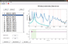 |
Figure 1. Graphical interface used for the proposed identification method. |
3.2 Definition of the identification window
Figure 2 shows the typical shape of a signal resulting from a short excitation, used as input for the method. The time t = 0 corresponds here to a moment when the system is at rest and has not yet received energy.
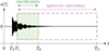 |
Figure 2. Definition of the time windows used for the identification of modal parameters and spectrum calculation. |
The time T0 denotes the onset of vibration. Although not used by the algorithm, T0 can be estimated, for example, by detecting when the signal exceeds a certain threshold relative to its maximum amplitude. When the vibration results from an impact applied to the structure, this impact has a finite duration, which depends on the contact stiffness between the exciter and the structure. As a result, the signal in the immediate vicinity of T0 does not strictly correspond to a free vibration, and the model of equation (1) does not rigorously apply in this region.
For this reason, the signal is analyzed starting from a time T1, chosen by the user (via the initial time field in the interface), sufficiently far from the onset of vibration to ensure that the structure is no longer under excitation and is vibrating freely, but not too far either if one aims to estimate components that decay rapidly and may quickly fall below the background noise level. The choice of the initial time is not critical and remains relatively intuitive. To assist the user, the interface updates the spectrum in real time whenever this time is modified.
The time T2 refers to a later instant than T1, such that the identification described in Section 2 is carried out over the interval [T1, T2]. From a user-interaction perspective, it is more convenient to define the duration of the interval rather than T2 itself; this is done using the window length field. Choosing this duration involves a trade-off. If it is too long, the number of samples K used for the identification increases, and the time required for the least-squares solution of equation (4), which is repeatedly performed during the optimization of each component, increases accordingly. If the duration is too short, the identification may lose accuracy, particularly when estimating the damping ratio of components that decay very slowly.
3.3 Spectrum calculation
To enable the identification method to operate with a peak-picking-like procedure, a spectrum is continuously displayed, as shown in Figure 1. It serves two purposes: selecting peaks corresponding to the components to identify, and monitoring the identification process by overlaying the reconstructed spectrum on top of the measured one. Each spectrum is computed using the Fast Fourier Transform (FFT) algorithm.
To compute the measured spectrum, the portion of the signal with t > T1 is used, so that the visible components are representative of those within the identification window. However, to benefit from good frequency resolution, the full portion from T1 to Tf (end of the signal) is used instead of just [T1, T2], as illustrated in Figure 2. Similarly, the reconstructed spectrum is also computed over [T1, Tf] so that both spectra are compared under identical conditions. This ensures that possible artifacts from the discrete Fourier transform, such as spectral leakage, appear similarly in both spectra. This also means that the reconstructed signal must be computed over a longer interval ([T1, Tf]) than the identification window ([T1, T2]). Far from being a minor implementation detail, the precise way both spectra are calculated and compared contributes to the reliability of the identification process from the user’s perspective.
3.4 User actions
3.4.1 Adding a component
To add a new component to the basis, the user is asked to select a visible peak on the spectrum. A component is then added to the signal model with an initial guess for the frequency and damping ratio, denoted ω0 and ξ0, after which these two parameters are adjusted by solving the minimization problem described by equation (11). The user’s selection provides the initial guess for the frequency, while the initial guess for the damping ratio is treated as a hidden parameter. It is currently fixed at 0.1% in the implementation. It has been observed that the minimization algorithm performs well with this value, even when the actual damping ratio differs by one or two orders of magnitude.
The peak selection is done using the function ginput in Matlab, which returns the coordinates of the point clicked in the display area. Specifically, the horizontal coordinate (the frequency at the location of the click) is used as the initial guess for the natural frequency. The minimization of the cost function involved in equation (11) is performed using the Nelder-Mead simplex algorithm, which is readily available in common scientific computing environments. The fminsearch function in Matlab is used here. In practice, to account for the potentially very different orders of magnitude of ωn and ξn, the optimization problem defined by equation (11) is preferably solved using dimensionless variables α and β, such that  and
and  represent the optimized parameters. Finding the amplitudes An and Bn within the cost function is straightforward since it results from solving a linear system of equations and is relatively inexpensive computationally. In practice, instead of using the expression in equation (8),
  is found by solving equation (4) in the least-squares sense, using the mldivide function in Matlab (or equivalently, the backslash operator). These operations are performed by the FindAmplitudes function, whose content is detailed in Algorithm 1.
It should be emphasized that the parameters of the newly added component (frequency, damping, amplitudes) are found while accounting for all other components already present in the basis, if any. Conversely, the amplitudes of all components previously included in the basis are simultaneously updated to reflect the influence of the newly introduced one. The full procedure to add a component is summarized in Algorithm 2.
3.4.2 Removing a component
It is sometimes necessary to remove a component from the basis. This typically occurs when the component addition procedure fails and results in a spurious component, i.e., a component that clearly does not correspond to a physical mode, but instead appears to have captured measurement noise or parasitic oscillations. In such cases, the user can select the undesired component from the list and execute the Remove action. The corresponding pair (ωn, ξn) is then removed from the basis, and the function FindAmplitudes is immediately called to update the amplitudes of the remaining components. These operations are summarized in Algorithm 3.
3.4.3 Refining the identification
This action consists in re-optimizing the frequency and damping ratio of each component currently included in the basis. Since the optimization problem defined by equation (11) is semi-local, the introduction of new components can alter the optimal parameters of previously added ones. The refinement action allows these parameters to be updated consistently, taking into account the influence of all components currently in the model. This operation is essential to ensure the robustness of the identification process, particularly under conditions of strong modal overlap, as illustrated later in Section 4.4. The refinement procedure is summarized in Algorithm 4.
4 Illustration of the method
As a test case, the method is applied to identify the natural frequencies and damping ratios of a stemmed wineglass based on the sound it radiates when struck. Due to its axisymmetric geometry, the structure exhibits eigenmodes with closely spaced frequencies, making it a representative case for evaluating the ability of the method to resolve such components.
4.1 Experimental setup
As this section also aims to demonstrate that the proposed procedure can operate with a simple measurement setup, the experimental protocol is deliberately kept minimal, as shown in Figure 3a A microphone (Roga MI21) is positioned 2 cm away from the structure and connected to an audio interface (Focusrite Scarlett 2i2). During the measurement, the scene is also recorded by a smartphone (Apple iPhone 6) located approximately 70 cm away. This provides two distinct time-domain signals for the same phenomenon: one captured by a Class 1 microphone typically used for high-quality acoustic measurements, and the other acquired using a widely available consumer device. The objective is to assess whether the identification method is robust enough to operate on a low-cost measurement.
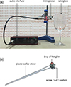 |
Figure 3. (a) Experimental setup to measure sound radiated by a struck wineglass. (b) Homemade flexible impact hammer to excite small structures for output-only measurements. |
To apply a clean, short-duration impact that efficiently excites the modes of interest, a homemade impact hammer was built. It is inspired by the miniature hammer PCB 086E80 used in the experiment described in Section 5, in that it features a flexible handle that helps prevent double impacts, although it obviously does not measure the impact force. As shown in Figure 3b, the hammer consists of a plastic coffee stirrer, weighted at one end by an M4 screw, nut, and washer assembly. A drop of hot glue has been applied to the head of the screw to provide a lower contact stiffness. Depending on which side is used for the impact (the metallic screw end or the glue drop) it is possible to produce either a harder or softer excitation, similar to changing the tip on a conventional impact hammer. This low-cost, homemade hammer proves to be a convenient tool for exciting small vibrating structures in such output-only measurement configurations. It should be noted that impact excitation inherently provides a limited bandwidth. The excitation bandwidth depends on the duration of the contact force, which is related to the hardness of the contact. While this bandwidth can be partially controlled through the selection of the impactor tip, it may in some cases be difficult to sufficiently excite high-frequency components. This limitation, inherent to the nature of impact excitation, may compromise the identification of such components. Alternatively, when appropriate, a broadband excitation may be provided by a simple plucking excitation (i.e., static loading followed by release).
Video 1 provided in the supplementary material shows the experiment being performed, while Sounds 1 and 2 correspond to the audio recorded simultaneously by the microphone and the smartphone, respectively.
4.2 Identification results
Figure 4a shows the time-domain signal measured by the microphone when the wineglass is struck. This is a typical free vibration response, characterized by a global amplitude decay over time. This decay is not monotonic: clear beating patterns appear, which is the signature of closely spaced frequency components.
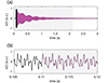 |
Figure 4. (a) Time-domain response of the wineglass excited by an impact, measured with the microphone. The black curve is the measured signal, while the colored curve is its reconstruction using the identified parameters. The shaded region indicates the portion of the signal used for identification. (b) Zoom on the beginning of the identification window. |
The corresponding spectrum is shown in Figure 5a. It exhibits five prominent components in the [0–8000] Hz range, each of which, when zoomed in, reveals a closely spaced pair of peaks (see Fig. 5b). These components very likely correspond to vibrational modes with deformation localized in the bowl of the glass [18], whose axisymmetric shape (imperfect in practice) results in doublets of modes with closely spaced frequencies. Several weaker components, visible as small, sharp peaks, can also be observed in the spectrum, for example at 1356 Hz and 2448 Hz. They probably correspond to other modes of the glass (such as torsional modes), which radiate sound less efficiently. These secondary components are not considered further, although they could be captured by the present identification approach.
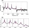 |
Figure 5. (a) Spectrum of the signal measured with the microphone (black) and of the reconstructed signal (colored), based on the identified parameters. (b) Zoom on each peak. The spectra are normalized to the amplitude of the maximum peak. |
The complete peak-picking procedure is illustrated in Video 2 provided in the supplementary material. The identification is performed over a window starting 40 ms after the onset of the vibrations captured by the microphone. As shown in the video, an observation window of 0.5 s is first used to allow for fast execution of the algorithm. Once the components are captured, the window is extended to 2 s and the identification is refined to improve accuracy. The spectrum reconstructed using the identified parameters is plotted in Figure 5. It closely matches the measured spectrum and accurately captures all doublets, including the last, weaker component.
The reconstructed time-domain signal is also plotted on Figure 4a. It accurately captures the overall amplitude envelope of the vibration. A closer look at the beginning of the identification window, as shown in the zoomed view in Figure 4b, reveals that the reconstructed signal closely matches the measured one. The small residual discrepancies can be attributed to low-frequency noise (below 100 Hz), whose spectral amplitude slightly exceeds that of the last identified component (see Fig. 5).
4.3 Robustness to noise
To jointly assess the robustness of the method to noise and its compatibility with simple recording equipment, an additional identification is performed using the audio signal recorded by the smartphone during the video.
The measured spectrum is shown in Figure 6a. The five main components of interest are clearly visible, but the signal-to-noise ratio is noticeably lower than with the dedicated measurement microphone. The zoomed views in Figure 6b reveal in particular that the last component barely emerges from the noise. Differences in the relative amplitudes of the two peaks within each doublet are also observed compared to the microphone measurement (Fig. 5b). This is especially noticeable for the doublets centered around 3353 Hz and 7387 Hz. Such differences are expected, as for a given excitation, the amplitude of each modal component in the measured signal depends on the location where the sound (or vibration) is captured. In addition, near the doublet centered around 1763 Hz, some components not related to the vibration of the glass are clearly visible. These parasitic components are not considered in the identification process.
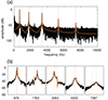 |
Figure 6. (a) Spectrum of the signal measured with the smartphone (black) and of the reconstructed signal (colored), based on the identified parameters. (b) Zoom on each peak. The spectra are normalized to the amplitude of the maximum peak. |
The peak-picking identification procedure is carried out similarly to the one applied to the microphone signal, using the same observation window. Video 3 provided in the supplementary material illustrates this procedure. The reconstructed spectrum obtained from the identified parameters is plotted in Figure 6. Once again, the identification process successfully captures the modal doublets, including the last one.
Figure 7 graphically compares the natural frequencies and damping ratios obtained from the two signals, while Table 1 provides the corresponding numerical values. A very good agreement is observed between the two measurement setups. It can be observed that the relative difference between the damping ratios identified from the microphone and the smartphone is larger for modes 9 and 10 than for the other modes. This behavior can be attributed to the lower signal-to-noise ratio of the smartphone measurement for these components, which results in a higher uncertainty in the estimated damping ratios. It should be noted, however, that this difference remains small (below 10%), so that even the noisier signal measured by the smartphone allows the frequency-dependent evolution of the damping ratio to be captured unambiguously. Although elucidating the physical origin of this frequency-dependent damping ratio is beyond the scope of this paper, the proposed identification method provides a convenient way to investigate such questions based on simple and non-intrusive measurements.
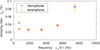 |
Figure 7. Frequencies and damping ratios of the 10 components identified from the microphone and smartphone signals. |
Natural frequencies ωn and damping ratios ξn of 10 modes of the wineglass, identified from the sound captured by the microphone or the smartphone. The relative differences indicated in parentheses and expressed as percentages are calculated with respect to the values identified by the microphone.
A complementary, more subjective evaluation of the method’s accuracy consists in comparing the measured sound with the synthesized one, generated from the identified parameters. This comparison is presented in Sounds 3 and 4 of the supplementary material, corresponding respectively to the recordings from the microphone and the smartphone. To ensure fair listening conditions, the comparison is made within the identification window (shaded region in Fig. 4a), which contains no significant component beyond 8000 Hz1. Each synthesized sound closely matches the original, except for the beneficial absence of background noise, particularly noticeable when comparing the smartphone recording and its synthesized version. The sound signature of the object, determined by its natural frequencies and damping ratios, is thus well captured. This identification procedure could therefore be used to create audio digital twins of musical instruments whose sound results from free oscillations. This would be particularly valuable for heritage instruments, such as antique bells [19], allowing their characteristic sound to be represented in the form of numerical parameters, which can serve as a reference for the production of faithful replicas.
4.4 Mutual dependency of component optimization
This section illustrates how the optimization of a component’s frequency and damping ratio depends on the other components already present in the basis, as mathematically expressed by equation (11). To this end, starting from an empty basis, we attempt to identify two closely spaced components around 5300 Hz, visible in the zoomed region of the spectrum shown in Figure 8a. For greater clarity, these components (or peaks) are referred to as A and B, as indicated in the figure.
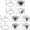 |
Figure 8. Evolution of the reconstructed spectrum over the four steps described in Section 4.4, along with the cost functions associated with the components of interest. |
The following four actions are successively performed in the interface:
-
adding a mode (component A),
-
adding a mode (component B),
-
refining the identification,
-
refining the identification again.
The paragraphs below comment on the result of each action. For better understanding, the reader is invited to refer to Video 4 provided in the supplementary material, which shows this sequence being performed in the interface.
After additional refinement steps, not discussed here for brevity but visible in the accompanying video, convergence is achieved.
5 Experimental validation
This section aims to demonstrate that the natural frequencies and damping ratios identified using the proposed method are consistent with those obtained through a more conventional modal analysis approach based on frequency response functions.
5.1 Experimental setup
Experiments were conducted on a rectangular medium-density fiberboard (MDF) plate. The choice of this material is motivated by its relatively high internal damping, which promotes modal overlap. The plate dimensions are 210 mm × 200 mm × 6 mm. Figure 9 shows the experimental setup. The plate is supported on four small foam blocks, approximating free boundary conditions. An accelerometer (PCB 352C23) is placed in one corner, and excitation is applied at the same location using a miniature impact hammer (PCB 086E80). A microphone (Roga MI21) is also positioned above the plate. Data acquisition is performed using a two-channel audio interface (Focusrite Scarlett 2i2).
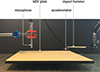 |
Figure 9. Experimental setup for the characterization of the MDF plate. |
Using this experimental setup, two types of data are successively acquired: first, a frequency response function computed from the force and acceleration signals, representative of a conventional modal analysis setup; and second, time-domain signals of acceleration and acoustic pressure in response to an unknown excitation. For convenience, this excitation is still applied using the impact hammer, but without recording the force signal, thus creating conditions that are just sufficient for the application of the proposed method.
5.2 FRF acquisition and data processing
To obtain the FRF, three impacts are successively applied to the structure within a single time acquisition. The corresponding raw signals from the force sensor and the accelerometer are provided in the supplementary material (Sound 5). For each impact, the excitation and response signals are extracted over a 2 s time window starting 0.01 s before the peak value of the force signal. The auto- and cross-spectra are estimated without any digital filtering or time-domain windowing of the excitation and response signals. This choice is motivated by the good signal-to-noise ratio of both signals and the short response duration due to the relatively high damping of the structure, making the force-exponential window commonly used in impact testing unnecessary. As a result, spectral leakage effects are not expected to influence the estimated FRF. The H1 estimator is used for FRF computation. It was verified that the choice of the estimator (H1, H2, or Hv) does not induce any noticeable difference in the resulting FRF, neither at resonances nor at anti-resonances. The pronounced damping observed at higher resonant frequencies is therefore attributed to the physical behavior of the structure rather than to the data processing or the choice of the FRF estimator. For the following analysis, the frequency range [0–3000] Hz is retained. Within this range, the force spectrum remains approximately flat, and the upper bound corresponds to a 10 dB drop in the input force spectral density due to the finite duration of the impact.
5.3 Modal identification from FRF
Figure 10a shows the measured mobility, defined as the ratio of velocity to force, at the excitation point. This mobility exhibits about twenty resonance peaks within the considered frequency range. These frequency-domain data are used to identify the natural frequencies and damping ratios by means of a frequency-domain identification method formulated under a MDOF assumption. The algorithm, detailed in [20], also relies on a peak-picking procedure and models the frequency response as:
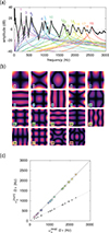 |
Figure 10. (a) Measured FRF (black) and reconstructed FRF (gray) using modal parameters identified with a frequency-domain method. The contribution of each mode is shown in color, along with the low-frequency and high-frequency residual terms (dashed lines). (b) Mode shapes computed using a finite element model. (c) Comparison between experimental and numerical natural frequencies before (dots) and after (stars) updating the Young’s modulus. |
 (12)
(12)
where Kn is a real-valued coefficient controlling the amplitude of each modal contribution.
A total of 19 modes are selected for identification, to which two additional components are added: a zero-frequency mode, acting as a low-frequency residual term that accounts for the mass contribution of rigid-body modes, and a deliberately introduced spurious mode at 5000 Hz with a damping ratio of 30%, acting as a high-frequency residual term that accounts for the stiffness contribution of modes beyond the identified range.
The mobility reconstructed by modal superposition using these 19 + 2 components matches the experimental data very closely, as shown in the same figure. The colored curves represent the contribution of each individual mode, clearly illustrating the significant modal overlap observed in some frequency regions. Indeed, the peak of certain individual modal contributions is noticeably offset from the peak observed in the total response. This is consistent with conditions where a SDOF approximation would not be valid.
To verify that no modes of the plate are missed during the modal identification process, the 19 experimentally identified natural frequencies are compared to those of the first 19 modes computed using a finite element model. The model is built with Comsol Multiphysics and employs solid elements. The material is assumed to be isotropic, with a density set to ρ = 789 kg/m3, estimated from the measured mass of the plate, and a Poisson’s ratio of ν = 0.3. Free boundary conditions are applied. In an initial computation, the Young’s modulus is arbitrarily set to E0 = 1 GPa. The computed mode shapes are shown in Figure 10b. The comparison between experimental and numerical natural frequencies is illustrated by the grey points in Figure 10c. These points are found to lie nearly along a straight line, indicating a good correspondence between the theoretical and experimental modes. A linear regression yields a coefficient A = 0.498 such that ωn(num) = Aωn(exp). Given the assumption of isotropic material, the natural frequencies scale with  , making it possible to compute an updated Young’s modulus E = E0/A
2 so that the numerical natural frequencies match the experimental ones. The colored stars in Figure 10c correspond to the updated model, with E = 4 GPa, showing good agreement with the experimental data.
, making it possible to compute an updated Young’s modulus E = E0/A
2 so that the numerical natural frequencies match the experimental ones. The colored stars in Figure 10c correspond to the updated model, with E = 4 GPa, showing good agreement with the experimental data.
In the following, the natural frequencies and damping ratios obtained from this FRF are considered as reference data, representative of a conventional modal analysis procedure, and are used to validate the proposed time-domain, output-only identification method.
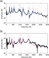 |
Figure 11. (a) Spectrum of the signal measured with the accelerometer (black) and its reconstruction (colored). (b) Spectrum of the signal measured with the microphone (black) and its reconstruction (colored). |
5.4 Modal identification from free responses
The spectra of free responses are presented in Figure 11a and 11b. The peak-picking procedure is applied to each of these signals, within a time window starting 10 ms after the onset of vibration and lasting 0.25 s. Video 5 in the supplementary material shows the identification process.
From the acceleration signal, all 19 components corresponding to the first 19 modes of the plate are successfully retrieved. Table 2 summarizes the identified natural frequencies and damping ratios. The identified natural frequencies match the reference values, with a deviation of less than 1% in most cases, except for mode 15, which clearly shows the strongest overlap with its nearest neighboring mode (see Fig. 10a). The identified damping ratios are also very close to the reference values. The largest discrepancy in damping is again observed for mode 15.
Natural frequencies ωn and damping ratios ξn of the first 19 modes of the MDF plate, identified using a frequency-domain method from an FRF, and the time-domain method from free vibration responses, either from acceleration (acc) or radiated sound (mic). The relative errors, expressed as percentages, are calculated with respect to the values identified from the FRF, which are taken as reference values.
From the microphone signal, only the first 12 components are successfully identified (see Fig. 11b). This is mainly due to the lower signal-to-noise ratio in this radiated sound measurement. Nevertheless, the identified frequencies and damping ratios show only very small deviations from the reference values (see Tab. 2).
Figure 12 provides a visual summary, in the frequency-damping plane, of the parameters identified by the peak-picking procedure applied to the time-domain acceleration and radiated sound signals, and how these parameters compare with the reference values obtained from frequency-domain identification. It is observed that the parameters identified from a single free response acceleration signal perform comparably to those obtained from a conventional FRF-based modal analysis. The modal updating process, consisting of pairing the modes and adjusting the Young’s modulus (as illustrated in Fig. 10c), could therefore have been successfully carried out using the natural frequencies identified from the free response. Moreover, although the identification from the radiated sound signal covers a limited frequency range in this case, it still allows for a reliable identification of the first structural modes. This demonstrates that the proposed identification method, combined with the simple and non-intrusive measurement of the sound radiated by the structure in response to an excitation that does not need to be controlled or quantified, is also suitable for identifying the natural frequencies and damping ratios.
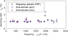 |
Figure 12. Frequencies and damping ratios of the 19 components identified from the accelerometer and microphone signals, compared with the FRF-based modal identification results. |
The present experimental validation also highlights a limitation of the method when modal overlap prevents a clear visual separation of individual components in the spectrum, either because a single peak contains contributions from two modes or because a component is masked by its neighboring components. In such cases, a mode may be easily overlooked without prior information indicating its presence. This is notably the case for mode 15, which does not manifest itself as a clearly identifiable peak in the spectrum shown in Figure 11a, despite being predicted by the finite element model and identified by FRF-based modal analysis. This limitation primarily concerns mode detectability rather than the ability of the algorithm to resolve overlapping components (such as components 11–12 and 14–15 in Fig. 11a).
6 Conclusion
This paper presented an output-only identification method for estimating natural frequencies and damping ratios from free vibration data. The approach combines the intuitive nature of peak-picking with the robustness of an MDOF formulation, through a parametric representation of the signal as a sum of damped sinusoids. The proposed approach was illustrated through experimental applications. It was shown to successfully resolve closely spaced frequency components and to remain robust in the presence of modal overlap and low signal-to-noise ratio. The method was also found to be applicable with a simple and non-invasive measurement setup, including cases where the identification is based solely on the sound radiated by the structure. Furthermore, the natural frequencies and damping ratios estimated with the method were consistent with those obtained from a more conventional FRF-based modal identification in the frequency domain.
This method naturally comes with some limitations. Due to its supervised nature, it is not well suited for cases where a very large number of modes need to be identified, as manually selecting many components from the spectrum would be time-consuming and cumbersome. In addition, the method in its current form does not provide direct access to mode shapes. However, since it accurately identifies the poles (i.e., natural frequencies and damping ratios), it can be used as a preliminary step for extracting residues from a set of frequency response functions, if available. These residues can then be used to reconstruct mode shapes.
Finally, by enabling the estimation of natural frequencies and damping ratios from a sound recorded on the fly through the interface, possibly using the computer’s built-in microphone, the method is well adapted for rapid assessments of damping properties without specialized equipment. This makes it a potentially helpful tool in instrument making, especially in guiding the choice of wood based on its damping characteristics. In this perspective, an open-access implementation of the method is currently in development, with the aim of making the interface broadly accessible without the need for proprietary software.
Conflicts of interest
The author declares no conflict of interest.
Data availability statement
Data are available on request from the authors.
Supplementary material
Audio and video files associated with Section 4
-
Sound 1 (mono, measured with the microphone): http://perso.univ-lemans.fr/~fablit/PeakPicking/WineGlass_Microphone_Measured.wav.
-
Sound 2 (mono, measured with the smartphone): http://perso.univ-lemans.fr/~fablit/PeakPicking/WineGlass_Smartphone_Measured.wav.
-
Sound 3 (mono, comparison between measured and synthesized sounds, from microphone recording): http://perso.univ-lemans.fr/~fablit/PeakPicking/WineGlass_Microphone_Comparison.wav.
-
Sound 4 (mono, comparison between measured and synthesized sounds, from smartphone recording): http://perso.univ-lemans.fr/~fablit/PeakPicking/WineGlass_Smartphone_Comparison.wav.
-
Video 1: http://perso.univ-lemans.fr/~fablit/PeakPicking/WineGlass_Experiment.mp4.
-
Video 2: http://perso.univ-lemans.fr/~fablit/PeakPicking/WineGlass_PeakPicking_Microphone.mp4.
-
Video 3: http://perso.univ-lemans.fr/~fablit/PeakPicking/WineGlass_PeakPicking_Smartphone.mp4.
-
Video 4: http://perso.univ-lemans.fr/~fablit/PeakPicking/WineGlass_MutualDependency.mp4.
Audio and video files associated with Section 5
-
Sound 5 (stereo, left: force sensor, right: accelerometer): http://perso.univ-lemans.fr/~fablit/PeakPicking/MDFplate_Force_Acc_3.wav.
-
Sound 6 (mono, measured with the accelerometer): http://perso.univ-lemans.fr/~fablit/PeakPicking/MDFplate_Accelerometer_Measured.wav.
-
Sound 7 (mono, measured with the microphone): http://perso.univ-lemans.fr/~fablit/PeakPicking/MDFplate_Microphone_Measured.wav.
-
Video 5: http://perso.univ-lemans.fr/~fablit/PeakPicking/MDFplate_PeakPicking_Accelerometer.mp4.
References
- K. Ege, N.B. Roozen, Q. Leclére, R.G. Rinaldi: Assessment of the apparent bending stiffness and damping of multilayer plates; modelling and experiment. Journal of Sound and Vibration 426 (2018) 129–149. [CrossRef] [Google Scholar]
- S. Vallely, S. Schoenwald: Higher-order modal parameter estimation and verification of cross-laminated timber plates for structural-acoustic analyses. Acta Acustica 8 (2024) 52. [Google Scholar]
- F. Soares, V. Debut, J. Antunes: The bar-resonator interaction in mallet percussion instruments: a multi-modal model and experimental validation. Journal of Sound and Vibration 548 (2023) 117528. [Google Scholar]
- M.S. Cao, G.G. Sha, Y.F. Gao, W. Ostachowicz: Structural damage identification using damping: a compendium of uses and features. Smart Materials and Structures 26 (2017) 043001. [Google Scholar]
- D.J. Ewins: Modal Testing: Theory, Practice and Application. John Wiley & Sons, 2000. [Google Scholar]
- J. He, Z.F. Fu: Modal Analysis. Butterworth-Heinemann, 2001. [Google Scholar]
- R. Allemang, P. Avitabile, Eds.: Handbook of Experimental Structural Dynamics. Springer, 2022. [Google Scholar]
- E. Foltête, M. Ouisse, G. Chevallier: Analyse modale expérimentale. Techniques de l’Ingénieur, 2025, Ref. R6180 v2. [Google Scholar]
- K. Ege, X. Boutillon, B. David: High-resolution modal analysis. Journal of Sound and Vibration 325 (2009) 852–869. [CrossRef] [Google Scholar]
- F.B. Zahid, Z.C. Ong, S.Y. Khoo: A review of operational modal analysis techniques for in-service modal identification. Journal of the Brazilian Society of Mechanical Sciences and Engineering 42 (2020) 398. [Google Scholar]
- C. Rainieri, G. Fabbrocino: Operational Modal Analysis of Civil Engineering Structures. Springer, 2014. [Google Scholar]
- B. Chomette, J.L. Le Carrou: Operational modal analysis applied to the concert harp. Mechanical Systems and Signal Processing 56, 57 (2015) 81–91. [Google Scholar]
- J.L. Le Carrou, A. Paté, B. Chomette: Influence of the player on the dynamics of the electric guitar. The Journal of the Acoustical Society of America 146 (2019) 3123–3130. [CrossRef] [PubMed] [Google Scholar]
- A. Paté, J.L. Le Carrou, B. Fabre: Predicting the decay time of solid body electric guitar tones. The Journal of the Acoustical Society of America 135 (2014) 3045–3055. [CrossRef] [PubMed] [Google Scholar]
- M. Géradin, D.J. Rixen: Mechanical Vibrations: Theory and Application to Structural Dynamics. Wiley, 2015. [Google Scholar]
- M. He, P. Liang, J. Liu, Z. Liang: Review and comparison of methods and benchmarks for automatic modal identification based on stabilization diagram. Journal of Traffic and Transportation Engineering (English Edition) 11 (2024) 209–224. [Google Scholar]
- R. Volkmar, K. Soal, Y. Govers, M. Böswald: Experimental and operational modal analysis: automated system identification for safety-critical applications. Mechanical Systems and Signal Processing 183 (2023) 109658. [Google Scholar]
- A.P. French: In vino veritas: a study of wineglass acoustics. American Journal of Physics 51 (1983) 688–694. [Google Scholar]
- M. Carvalho, V. Debut, J. Antunes: Physical modelling techniques for the dynamical characterization and sound synthesis of historical bells. Heritage Science 9 (2021) 157. [Google Scholar]
- F. Ablitzer: Peak-picking identification technique for modal expansion of input impedance of brass instruments. Acta Acustica 5 (2021) 53. [CrossRef] [EDP Sciences] [Google Scholar]
Appendices
Appendix A Algorithms
Input: Time vector t = [t1, …, tK]T and sampled signal y = [s(t1),…,s(tK)]T in the identification window (see Fig. 2), list of natural frequencies ω = [ω1, …, ωN] and damping ratios ξ = [ξ1, …, ξN]
Output: Amplitudes An and Bn, residual error R
-
Compute the damped natural frequencies:

for n ∈ [1, …, N]
-
Construct matrix A (K lines, 2N columns) defined by equation (5)
-
Solve the least-squares problem:
(e.g. using mldivide function in Matlab)
-
Extract the amplitudes:
![Mathematical equation: $$ A_1 = \mathbf{\widehat{x} }[1], \ldots , A_N = \mathbf{\widehat{x} }[N] \quad \text{ and} \quad B_1 = \mathbf{\widehat{x} }[N+1], \ldots , B_N = \mathbf{\widehat{x} }[2N] $$](/articles/aacus/full_html/2026/01/aacus250111/aacus250111-eq20.gif)
-
Compute the residual error:
-
Prompt the user to select an initial frequency guess from the spectrum of the signal (e.g. using ginput function in Matlab)
-
Set initial values for the new component
-
Optimize the new component:
where
![Mathematical equation: $$ R(\alpha ,\beta ) = \mathtt FindAmplitudes \left(\mathbf t , \mathbf y , \left[\widehat{\omega }_1,\cdots ,\widehat{\omega }_N,\alpha \cdot \omega _0\right], \left[\widehat{\xi }_1,\cdots ,\widehat{\xi }_N,\beta \cdot \xi _0\right] \right) $$](/articles/aacus/full_html/2026/01/aacus250111/aacus250111-eq24.gif)
(e.g. using fminsearch function in Matlab)
-
Update the list of frequencies and damping ratios
![Mathematical equation: $$ \begin{aligned}&\boldsymbol{\omega } \leftarrow \left[\widehat{\omega }_1,\cdots ,\widehat{\omega }_N,\widehat{\alpha } \cdot \omega _0\right] \\&\boldsymbol{\xi } \leftarrow \left[\widehat{\xi }_1,\cdots ,\widehat{\xi }_N,\widehat{\beta } \cdot \xi _0\right] \end{aligned} $$](/articles/aacus/full_html/2026/01/aacus250111/aacus250111-eq25.gif)
-
Sort the elements in ω and ξ by ascending order of frequency
-
Update the amplitudes:

-
Synthesize the signal with equation (2) and compute its spectrum
-
Udpate display: refresh the list, time-domain and frequency-domain plots
-
Assign to n the index of the component currently selected in the list
-
Remove the n-th component from the basis
![Mathematical equation: $$ \begin{aligned}&\boldsymbol{\omega } \leftarrow \left[ \widehat{\omega }_1, \dots , \widehat{\omega }_{n-1}, \widehat{\omega }_{n+1}, \dots , \widehat{\omega }_{N}\right]\\&\boldsymbol{\xi } \leftarrow \left[ \widehat{\xi }_1, \dots , \widehat{\xi }_{n-1}, \widehat{\xi }_{n+1}, \dots , \widehat{\xi }_{N}\right] \end{aligned} $$](/articles/aacus/full_html/2026/01/aacus250111/aacus250111-eq27.gif)
-
Update the amplitudes:

-
Synthesize the signal with equation (2) and compute its spectrum
-
Udpate display: refresh the list, time-domain and frequency-domain plots
-
for n = 1 to N do
-
Optimize the n-th component:
where
![Mathematical equation: $$ R(\alpha ,\beta ) = \mathtt FindAmplitudes \left( \mathbf t , \mathbf y , \left[\widehat{\omega }_1,\cdots ,\alpha \cdot \widehat{\omega }_n,\cdots ,\widehat{\omega }_N\right], \left[\widehat{\xi }_1,\cdots ,\beta \cdot \widehat{\xi }_n,\cdots ,\widehat{\xi }_N\right] \right) $$](/articles/aacus/full_html/2026/01/aacus250111/aacus250111-eq30.gif)
(e.g. using fminsearch function in Matlab)
-
Update the list of frequencies and damping ratios
![Mathematical equation: $$ \begin{aligned}&\boldsymbol{\omega } \leftarrow \left[\widehat{\omega }_1,\cdots ,\widehat{\alpha } \cdot \widehat{\omega }_n,\cdots ,\widehat{\omega }_N\right] \\&\boldsymbol{\xi } \leftarrow \left[\widehat{\xi }_1,\cdots ,\widehat{\beta } \cdot \widehat{\xi }_n,\cdots ,\widehat{\xi }_N\right] \end{aligned} $$](/articles/aacus/full_html/2026/01/aacus250111/aacus250111-eq31.gif)
-
end for
-
Sort the elements in ω and ξ by ascending order of frequency
-
Update the amplitudes:

-
Synthesize the signal with equation (2) and compute its spectrum
-
Udpate display: refresh the list, time-domain and frequency-domain plots
The full measured signal, i.e., for t ∈ [0, Tf] (Sounds 1 and 2), contains higher frequency components, resulting in a brighter attack.
Cite this article as: Ablitzer F. 2026. Peak-picking method for identifying natural frequencies and damping ratios from free vibration measurements. Acta Acustica, 10, 18. https://doi.org/10.1051/aacus/2026014.
All Tables
Natural frequencies ωn and damping ratios ξn of 10 modes of the wineglass, identified from the sound captured by the microphone or the smartphone. The relative differences indicated in parentheses and expressed as percentages are calculated with respect to the values identified by the microphone.
Natural frequencies ωn and damping ratios ξn of the first 19 modes of the MDF plate, identified using a frequency-domain method from an FRF, and the time-domain method from free vibration responses, either from acceleration (acc) or radiated sound (mic). The relative errors, expressed as percentages, are calculated with respect to the values identified from the FRF, which are taken as reference values.
All Figures
|
Figure 1. Graphical interface used for the proposed identification method. |
| In the text | |
|
Figure 2. Definition of the time windows used for the identification of modal parameters and spectrum calculation. |
| In the text | |
|
Figure 3. (a) Experimental setup to measure sound radiated by a struck wineglass. (b) Homemade flexible impact hammer to excite small structures for output-only measurements. |
| In the text | |
|
Figure 4. (a) Time-domain response of the wineglass excited by an impact, measured with the microphone. The black curve is the measured signal, while the colored curve is its reconstruction using the identified parameters. The shaded region indicates the portion of the signal used for identification. (b) Zoom on the beginning of the identification window. |
| In the text | |
|
Figure 5. (a) Spectrum of the signal measured with the microphone (black) and of the reconstructed signal (colored), based on the identified parameters. (b) Zoom on each peak. The spectra are normalized to the amplitude of the maximum peak. |
| In the text | |
|
Figure 6. (a) Spectrum of the signal measured with the smartphone (black) and of the reconstructed signal (colored), based on the identified parameters. (b) Zoom on each peak. The spectra are normalized to the amplitude of the maximum peak. |
| In the text | |
|
Figure 7. Frequencies and damping ratios of the 10 components identified from the microphone and smartphone signals. |
| In the text | |
|
Figure 8. Evolution of the reconstructed spectrum over the four steps described in Section 4.4, along with the cost functions associated with the components of interest. |
| In the text | |
|
Figure 9. Experimental setup for the characterization of the MDF plate. |
| In the text | |
|
Figure 10. (a) Measured FRF (black) and reconstructed FRF (gray) using modal parameters identified with a frequency-domain method. The contribution of each mode is shown in color, along with the low-frequency and high-frequency residual terms (dashed lines). (b) Mode shapes computed using a finite element model. (c) Comparison between experimental and numerical natural frequencies before (dots) and after (stars) updating the Young’s modulus. |
| In the text | |
|
Figure 11. (a) Spectrum of the signal measured with the accelerometer (black) and its reconstruction (colored). (b) Spectrum of the signal measured with the microphone (black) and its reconstruction (colored). |
| In the text | |
|
Figure 12. Frequencies and damping ratios of the 19 components identified from the accelerometer and microphone signals, compared with the FRF-based modal identification results. |
| In the text | |
Current usage metrics show cumulative count of Article Views (full-text article views including HTML views, PDF and ePub downloads, according to the available data) and Abstracts Views on Vision4Press platform.
Data correspond to usage on the plateform after 2015. The current usage metrics is available 48-96 hours after online publication and is updated daily on week days.
Initial download of the metrics may take a while.