| Issue |
Acta Acust.
Volume 10, 2026
|
|
|---|---|---|
| Article Number | 36 | |
| Number of page(s) | 24 | |
| Section | Environmental Noise | |
| DOI | https://doi.org/10.1051/aacus/2026032 | |
| Published online | 12 May 2026 | |
Scientific Article
Human response to air source heat pump noise: influence of background noise, operating conditions and acoustic characteristics
Salford Acoustics Innovation Institute, University of Salford, Manchester M5 4WT, United Kingdom
* Corresponding author: This email address is being protected from spambots. You need JavaScript enabled to view it.
Received:
26
September
2025
Accepted:
3
April
2026
Abstract
Air Source Heat Pumps (ASHPs) are key to reducing carbon emissions from heating requirements of buildings, especially in colder regions like Europe. However, installation rates remain below targets, with noise emissions posing a major barrier to wider adoption in residential areas. This study examines human response to ASHP noise under simulated conditions, focusing on Annoyance, Arousal, and Valence under varying source distances, background noise levels, and operating conditions, emphasising changes in the acoustic characteristics of the heat pump. A two-part listening experiment was conducted with 50 participants. Part One evaluated responses to continuous ASHP noise using 20-second recordings. Part Two focused on transient operating conditions, utilising 60-second recordings where the heat pump transitioned between operating modes. Recordings combined ASHP noise at three distinct source distances with two ambient background noise levels, simulating rural day- and nighttime scenarios. A contextual framing condition regarding ASHP ownership was also included. Results show that higher A-weighted Sound Pressure Level (SPL), Loudness, Roughness, and Tonality are associated with increased Annoyance and Arousal and decreased Valence. Correlation analysis revealed that conventional metrics (SPL) and psychoacoustic parameters (particularly Loudness and Roughness) show similar strength associations with subjective responses, with their relative importance varying across different experimental conditions. These results suggest that while conventional A-weighted sound level measurements remain important, ASHP noise regulations might benefit from additionally considering psychoacoustic characteristics. Simulated background noise suggests ASHP noise perception interacts with ambient conditions, but field studies with realistic background noise are needed to guide regulation.
Key words: Psychoacoustics / Environmental noise / Air source heat pumps / Heat pump noise / Human response to noise
© The Author(s), Published by EDP Sciences, 2026
 This is an Open Access article distributed under the terms of the Creative Commons Attribution License (https://creativecommons.org/licenses/by/4.0), which permits unrestricted use, distribution, and reproduction in any medium, provided the original work is properly cited.
1 Introduction
The global heat pump market has expanded significantly over the past few years. Air Source Heat Pumps (ASHPs) have emerged as a viable alternative for consumers seeking to replace traditional fossil fuel heating systems. They are promoted as low-maintenance, cost-effective solutions that are more efficient than fossil fuel-based gas boilers [1, 2], and can contribute significantly to reducing carbon emissions.
In Europe, 40% of the energy is consumed by buildings, making them the continent’s single largest source of energy consumption. The vast majority of these buildings are not energy efficient and are powered by fossil fuels, which create 36% of Europe’s greenhouse gas emissions [3]. According to 2022 data from the International Energy Agency (IEA), Europe’s contribution to global carbon emissions from combustible fuels is 10.5%, making the region the third-largest contributor to global carbon emissions after China and the United States [4]. Even though combustible fuels are not exclusively used for domestic needs, replacing fossil fuel-based systems with renewable systems such as the ASHPs plays an important role in decarbonising domestic heating and air conditioning, particularly in temperate and cold-climate regions where heating demands are substantial.
ASHPs extract heat from the outside air using a refrigerant fluid circling within a closed loop. This refrigerant is then compressed, raising its temperature, before passing through a heat exchanger or coil, where the heat is transferred to the water or air that heats the building. This process is completely reversible, allowing some types of ASHP to be used for cooling needs in addition to space heating or domestic hot water production [5]. Since this process is significantly more efficient than gas, biomass, or electrical boilers, ASHPs can significantly reduce electricity demand. Moreover, if this electricity is sourced from renewable energy, it can further reduce the negative climate impacts [6].
As part of efforts to meet the EU’s sustainability goals, consistent subsidies are provided to promote the installation of heat pumps. These efforts resulted in considerable growth in heat pump installations [7]. In 2023, 2.63 million heat pump units were installed across the EU, which was a significant increase compared to the 0.71 million installations in 2013 [8].
Ensuring positive attitudes towards heat pumps among end users is essential to sustain this trend. However, despite all their advantages, several factors have restricted the broader adoption of ASHPs. The UK Government, the UK Government has an ambitious target of 600 000 annual ASHP installations by 2028 to support Net Zero, but yearly installations are significantly below this target. Currently, one of the primary challenges for broader adoption and maintaining the upward trend in installations is addressing the end-users’ concerns about noise emissions [9, 10]. If overlooked, this problem could hamper the transition to renewable energy technologies.
The IEA has launched a Technology Collaboration Programme on Heat Pump Technologies (HPT) to address these concerns and maintain momentum. One of the Annexes launched by the IEA HPT was “Annex 51: Acoustic Signature of Heat Pumps”. This Annex ran between 2017 and 2020, with the participation of six countries, and focused on increasing the acceptance of heat pumps for comfort purposes concerning noise and vibration emissions [11]. Following the success of Annex 51, a new annex is underway, named “Annex 63: Placement Impact on Heat Pump Acoustics”, with the participation of eight countries [12].
The installation of ASHPs is closely regulated by frameworks that set specific criteria to ensure minimal adverse effects on the surrounding dwellings. Some of these criteria are sound emissions, unit sizes and location. For example, in the UK, ASHP installations are qualified under Permitted Development Rights (PDR), which allows them to be installed without planning permission if they comply with sound emissions outlined in the Microgeneration Certification Scheme (MCS) 020 a) [13]. This framework specifies that ASHP sound pressure levels (SPLs) must not exceed 37 dB(A), measured one meter away from the nearest window or door of a habitable room of a neighbouring property. However, at the time of writing, this method does not account for background noise levels, which may vary across different environments, such as urban versus rural areas. As a result, ASHPs in quieter locations may be perceived as disproportionately loud, while those in noisier areas might face unnecessary restrictions, further slowing down the adoption of this technology.
The acoustic character of an ASHP’s noise emissions is an essential factor influencing its impact on wellbeing. While regulations typically address overall SPL, the distinctive spectral, temporal and psychoacoustical characteristics of ASHP noise require additional consideration to fully understand their effects on human perception and annoyance. The primary noise sources in an ASHP are the fan and compressor. The noise spectrum of a unit varies depending on the operation frequency of these components, which emit both broadband and tonal components [14]. These tonal components are typically observed at the blade passing frequency and higher-order harmonics [15]. Tonality can contribute significantly to the annoyance caused by ASHP operation. Hence, sound levels cannot adequately characterise noise annoyance; the acoustic character must be considered to understand the human response fully. In the UK, the assessment of industrial and commercial sounds requires consideration of the acoustic character in accordance with BS 4142:2014+A1:2019 [16] and includes a tonality penalty depending on the tone’s prominence. However, this assessment does not apply to ASHPs installed under the PDR and only applies to equipment installed under a general planning system [9]. Several European countries, such as Germany, Finland, and the Netherlands, also include tonal penalties in their noise assessment regulations [17]. For example, in Germany, there are tonal penalties based on an assessment by an acoustics expert, with the permitted levels reduced by 0 dB(A), 3 dB(A), or 6 dB(A), depending on the prominence of the tone [9].
While some countries have adopted more sophisticated noise assessment methodologies, such as the inclusion of tonal penalties, others continue to rely on frameworks that do not adequately account for perceptually salient acoustic features. A case study by Torjussen [10] highlights these shortcomings in the UK context. Despite meeting the permitted development noise limits, ASHPs were found to cause significant adverse impacts due to tonal noise characteristics. The author highlights that the UK’s current assessment methodology does not incorporate such acoustic features, increasing the risk of community noise complaints. The study proposed a revised procedure that includes tonality corrections to improve siting decisions and encourage manufacturers to address tonal emissions.
Stürenburg et al. [18] investigated the annoyance ratings of air-to-water heat pump noise, focusing on the differences between perceived loudness and preference across various operating states. Their findings revealed a discrepancy between loudness and preference, influenced significantly by the current operating states.
A study conducted as part of the IEA HPT Annex 51 [19, 20] investigated the annoyance response to ASHP noise through listening tests with Austrian and Swedish participants. Using 5-second-long samples and analysis of psychoacoustic parameter values, the researchers found that sound levels, loudness, sharpness, and roughness significantly influenced annoyance ratings. They also observed a directional dependence of noise effects, emphasising the importance of heat pump placement. A stepwise linear regression model developed in the study identified LAF50 (A-weighted sound level, fast time weighting, 50% exceedance level) as the best predictor, explaining approximately 87% of the variance in annoyance ratings. Additional parameters–peak loudness level (LN5), peak sharpness (S5), and peak roughness (R5)–contributed incrementally, with LN5 and S5 adding 5% and 3% of explained variance, respectively. While some parameters, such as loudness, roughness, and sharpness, offer insight into the perception of ASHP noise, the findings demonstrate that no single acoustic descriptor can fully account for annoyance responses, highlighting the need for models incorporating multiple parameters. Beyond annoyance, ASHP noise may also impact health-related outcomes such as sleep disturbance, particularly in residential settings. Environmental noise, even at moderate levels, is a recognised risk factor for sleep disruption, which can lead to longer-term cardiovascular and cognitive effects [21, 22]. Emerging research demonstrates that ASHP noise can adversely affect sleep and daytime functioning [23]. Laboratory studies using polysomnography reveal increased arousal rates during sleep under partially open window conditions compared to closed windows, alongside daytime increases in annoyance, concentration difficulties, and mood disturbances. These findings underscore the need to evaluate ASHP noise impacts under realistic propagation scenarios.
The noise from ASHPs will likely impact communities, and if not appropriately addressed, this could lead to tension within the exposed communities, further impacting acceptance. Finding a balance that minimises ASHPs’ environmental impact while avoiding overly restrictive policies to promote broader adoption and acceptance is crucial. Achieving this balance requires a shift from focusing solely on sound pressure metrics. Instead, it should involve combining objective measurements with subjective evaluations to better understand how people respond to ASHP noise.
The objective of this study is to use quantitative research methods to deepen the understanding of human response to ASHP noise and thereby guide policy. A two-part experiment is carried out for this purpose. Part One evaluates individuals’ reactions to Continuous ASHP operation under different source distances and varying ambient background noise conditions, simulating different ASHP placements and the daytime-nighttime noise levels typical of a rural area. Part Two assesses human responses to ASHP noise under variable operation, exploring how people react to transitions in operating conditions and stationary states.
-
1.
How do variations in ambient Background Noise levels relative to ASHP noise emissions influence human responses regarding reported Annoyance, Arousal, and Valence?
-
2.
How does the psychoacoustic character of the ASHP noise affect human response?
-
3.
Which acoustic and psychoacoustic parameters (e.g. sound level, loudness, roughness, sharpness, fluctuation strength, and tonality) predict human responses to ASHP noise, particularly regarding Annoyance, Arousal, and Valence?
-
4.
How does perceived ownership of the noise source influence reported affective responses to ASHP noise?
-
5.
How do transient conditions in the ASHP operation cycle affect human responses?
-
6.
What are the differences in Annoyance, Arousal, and Valence responses to continuous versus transient ASHP signals?
2 Methods
This experiment simulated a series of scenarios to investigate how people react to noise emissions from ASHPs placed at different distances outside their homes during different times of the day. The experiment was separated into two parts, which were concerned with ASHP noise under continuous and variable operating conditions. The first part measured human responses to 20-second-long continuous ASHP noise recordings. The second part focused on responses to ASHP noise emissions under variable operation using 60-second recordings, with participants evaluating their experience at two points: after a change in the operating conditions and at the end of the recording. The audio stimuli for the experiment consisted of ASHP noise samples under various operating conditions, combined with ambient background noise samples representative of daytime and nighttime scenarios.
2.1 ASHP noise samples
The ASHP noise samples used in this study were taken from two longer recordings, each lasting eight minutes and thirty-four seconds. These recordings were part of an acoustic holography project [20] conducted as part of the IEA HPT Annex 51 [11]. The recordings were made in a climate-controlled chamber with sound-absorbing walls and a reflective floor. This specialised environment minimises typical low-frequency challenges such as room modes and standing waves. A total of 64 microphones were arranged in a hexagonal prism configuration to capture the noise from a prototype air-to-water ASHP unit at a sampling rate of 96 kHz. For this study, two recordings were selected based on data from a microphone positioned in front of the fan outlet, 177.6 cm above the ground. While this is consistent with the standardised measurement protocol, this setup does not account for potential directivity effects of the ASHP noise, which may influence perceived acoustic characteristics depending on the listener’s position relative to the unit. These recordings captured the transitions in operating conditions, with the fan and compressor shifting between different power levels and frequencies. MATLAB R2023a was used to calibrate the recordings to their original sound levels using the provided 94 dB(A) 1 kHz calibration tone.
Audacity was used to trim the two longer recordings into 20-second and 60-second segments. The 20-second recordings, referred to as “Continuous,” were used in Part One of the experiment. These consisted of uninterrupted recordings of three distinct ASHP operating conditions (Fig. 1, top example): Minimum Capacity (Defrost), Moderate Capacity, and Maximum Capacity. The Defrost cycle is the most distinct of the three operating conditions, as the unit operates in reverse with only the compressor active, without any noise from the fan. Under normal operation, fan emissions can mask noise from other components of the unit, but their absence during Defrost produces a unique acoustic signature, often characterised by more pronounced tonal components [24]. Multiple segments were selected from the recordings for each condition and trimmed, resulting in a total of 14 initial samples (Minimum Capacity = 5, Moderate Capacity = 4, and Maximum Capacity = 5). The highly time-variant 60-second samples, referred to as “variable operation,” were used in Part Two of the experiment. These samples captured transitions between operating conditions, primarily from Maximum to Minimum (Max-to-Min) and from Minimum to Maximum (Min-to-Max) capacity, which can be categorised as dynamic cycles (Fig. 1, bottom example). Additionally, excerpts from steady operating conditions, referred to as “Stationary,” were selected to compare against dynamic cycles. This process yielded 10 initial samples of variable operation conditions for Part Two (Maximum to Minimum = 4, Minimum to Maximum = 4, Stationary = 2).
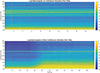 |
Figure 1. Log-spectrograms comparing a continuous ASHP stimulus (Part One) and a variable operation stimulus (Part Two), including a transition from minimum to maximum capacity. |
2.2 Ambient background noise samples
The ambient background noise levels of a rural area were selected for the study, with daytime levels at 39.5 dB(A) and nighttime levels at 31.5 dB(A) [25]. However, shaped pink noise was employed instead of using recordings of rural soundscapes. This method provided greater control over the stimuli, eliminating uncontrolled variables such as natural sounds (e.g. bird calls, wind) and anthropogenic noises (e.g. human speech). The ambient background noise was prepared by first generating pink noise in Audacity and then applying a filter curve using the Spectrum No. 2 defined in BS EN ISO 717-2020 [26], which specified one-third octave band levels representing a standardised traffic noise profile. This enabled the approximation of the spectral shape of urban traffic noise while avoiding the presence of recognisable natural or human-generated sounds that could influence perceptual responses. The shaped pink noise that simulated the traffic noise spectrum was exported with two durations–20 and 60 s–for use in different parts of the experiment.
2.3 Audio calibration and reproduction
Figure 2 shows the workflow used to prepare the audio stimuli. The original ASHP recordings were first calibrated to represent three source-to-receiver distances: 5, 10, and 15 m. These corresponded to target SPLs of 46 dB(A), 40 dB(A), and 36.5 dB(A), respectively, based on free-field attenuation from a ground-mounted source with a directivity factor of Q = 4. All SPL targets were referenced to a position 1 m in front of a building façade, following the UK MCS 020 a) installation standard [13].
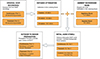 |
Figure 2. Diagram illustrating the preparation of the audio stimuli through calibration and reproduction. |
Ambient background noise samples were also calibrated to represent typical rural conditions: 39.5 dB(A) for daytime and 31.5 dB(A) for nighttime. These target levels were selected to simulate plausible outdoor background levels for the residential contexts considered [25]. Calibration was conducted in the Listening Room of the University of Salford’s Acoustic Laboratories. The playback system included an HP Omen 16 laptop, Motu 4Pre audio interface, Genelec 8030A loudspeaker, and 7020B subwoofer. According to the manufacturer’s specifications, the Genelec 8030A loudspeaker has a free-field frequency response of 58 Hz–20 kHz (±2 dB), with cut-off frequencies of < 55 Hz and > 21 kHz at −3 dB, while the Genelec 7050B subwoofer reproduces frequencies from approximately 25 Hz to 85 Hz (±3 dB). The combined playback system therefore reproduced frequencies from approximately 25 Hz to 21 kHz. To reflect the measurement procedure outlined in MCS 020 a) [13], a PCB Piezotronics free-field microphone was positioned 1 m from the loudspeaker on axis at a height of 1.2 m. Playback was controlled using Audacity, and SPLs were monitored using a Dewesoft SIRIUSi-8xACC data acquisition system and a Brüel & Kjær 2250 Class 1 sound level meter (SLM).
Each ASHP recording was played at reference gain and adjusted iteratively to achieve the LAeq, 20 s and LAeq, 60 s values matching the target levels, following a procedure similar to the one used by Torija and Flindell [27]. This process produced three calibrated versions of each ASHP recording, corresponding to the three source distances. Ambient background noise samples were calibrated to their respective targets, following the same procedure.
To generate the final stimuli, background noise was added to the distance-attenuated ASHP recordings using a Python script. For Part One, both daytime and nighttime ambient background noise conditions were mixed with each ASHP recording at each distance, resulting in a set of 84 stimuli (14 ASHP recordings × 3 distances × 2 background levels). For Part Two, only the nighttime background condition was used, resulting in a set of 30 stimuli (10 ASHP recordings × 3 distances × 1 background level). The exclusion of daytime background noise in Part Two was intended to limit test duration and participant fatigue [28].
To simulate indoor listening conditions, all final stimuli were filtered using the octave-band transmission loss curve for a partially open timber window “Window G” configuration, (50 000 mm2 opening) from [29] (Appendix B, Fig. B.1). This introduced realistic spectral shaping without additional environmental filtering such as atmospheric absorption, which was deemed negligible given the low-frequency content and short simulated propagation distances.
Final SPL verification was performed using the Dewesoft and further confirmed with the SLM, and stimuli were remeasured at the start of each test day. Any deviation greater than 0.5 dB(A) from the calibration levels was corrected. For both parts of the experiment, participants were exposed to half of the stimuli from each set. Stimuli were pseudo-randomised via a Python script to ensure balanced representation, with each item repeated 25 times across the full participant sample of 50.
2.4 Experimental procedure
The experimental methodology and data collection procedures were approved by the Ethics Committee of the University of Salford (ref. no. 2024-0145-228). Before starting the experiment, participants were divided into two groups of 25 to evaluate different ownership scenarios. They were instructed to imagine themselves sitting on their living room sofa, where, in addition to the usual household sounds, they could hear the noise of an ASHP through a partially open window. The first 25 participants were informed that the ASHP belonged to them (Scenario 1), while the remaining 25 were given no information about the ownership of the ASHP (Scenario 2), only that there was an ASHP outside. This distinction was made to see whether the ownership information would influence their responses to the noise.
Each participant listened to a total of 60 audio stimuli. For Part One, participants were presented with two control stimuli and 42 Continuous stimuli pseudo-randomly sampled from a total pool of 84 stimuli. The control stimuli only included shaped pink noise representing the ambient background noise. For Part Two, participants were presented with one control stimulus representing nighttime rural ambient background noise and 15 stimuli containing stationary conditions and transitions between maximum and minimum operational states, pseudo-randomly sampled from a pool of 30 stimuli. This sampling was balanced across the 50 participants for both parts to ensure that each stimulus in the total pool was evaluated by exactly 25 participants.
The experiment took place in the Listening Room using the audio reproduction system detailed in Section 2.3 and with the layout illustrated in Figure 3. The participants were seated at 2 m from the loudspeaker, corresponding to a plausible indoor listening position. This reproduction setup was designed to reflect typical indoor exposure to ASHP noise rather than the 1 m façade measurement location defined by MCS 020 a) [13]. Python’s PyQt 5 library was used to prepare the experimental Graphical User Interface (GUI). The experiment GUI was displayed on a screen placed directly above the loudspeaker.
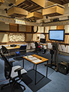 |
Figure 3. The layout of the Listening Room during the calibration process and the listening experiments. During calibration, the microphone is positioned 1 m away from the centre of the loudspeaker cone. The position above illustrates the distance for the listening experiment, which is 2 m from the loudspeaker cone. |
To assess individual differences in auditory perception, a questionnaire based on the Noise-Sensitivity-Questionnaire (NoiSeQ) [30] was sent to participants to complete before listening tests. The English translation of this questionnaire was verified before the experiment by directly reaching out to the authors of the original article. The NoiSeQ consists of five subscales: Communication, Work, Leisure, Habitation and Sleep, each containing five questions, for a total of 35 questions. However, one question from the Communication subscale was inadvertently omitted during the listening tests. Despite this, the calculation of global noise sensitivity scores, which involves reversing certain specific questions, summing the responses, and dividing by the total number of questions (34), remains unaffected. Additionally, while the original NoiSeQ used a 4-point scale from 0 to 3, a 5-point scale from 1 to 5 (1- Strongly disagree, 5-Strongly agree) was used instead to capture more granularity in the data and improve sensitivity.
Upon entering the Listening Room, each participant signed a consent form and completed a general demographics questionnaire. Before each part of the experiment, participants were given a short training session to familiarise themselves with the GUI and the terms used. The training session used four stimulus examples for Part 1 and two for Part 2, selected to represent the highest and lowest sound levels in the experiment. Participants were informed that these examples were chosen to reflect the range of levels they would encounter.
Part One of the experiment used Continuous recordings of ASHP noise, with the main aim of measuring peoples’ response to ASHP operation noise under different background noise levels (39.5 dB(A) daytime and 31.5 dB(A) nighttime) and source distances (46 dB(A) at 5 m, 40 dB(A) at 10 m and 36.5 dB(A) at 15 m). Each participant listened to 44 stimuli and evaluated their experience after each one by answering three questions. The first two of these questions were based on the Valence and Arousal dimensions of the pictorial scale of Self-Assessment Manikin (SAM) [31], measured on a nine-point scale.
Valence and Arousal are two dimensions of the circumplex model of affect [32], commonly used to describe emotional responses. Valence refers to the intrinsic pleasantness or unpleasantness of a stimulus, ranging from positive (pleasant) to negative (unpleasant). Arousal indicates the intensity of emotional activation, ranging from calm or sleepy to highly alert or excited. Together, they provide a continuous two-dimensional space for characterising affective states. These dimensions are also related to the Pleasantness and Eventfulness constructs in ISO 12913-2:2018 [33], which are used in soundscape research. The work by Axelsson et al. [34], which informed the development of ISO 12913-2, builds on Russell’s circumplex model of affect.
The third question measured the Annoyance towards the ASHP noise emissions using a 0-to-10 opinion scale. This question was based on the ISO/TS 15666:202 [35] which asked the participants to rate their annoyance by answering, “Thinking about the sound environment you just listened to, what number from 0 to 10 best represents the extent to which you are bothered, annoyed, or disturbed by the air source heat pump noise? (0- “Not Annoying at all”, 10- “Extremely Annoying”).” Once Part One was over, participants were advised to take a short break before proceeding to Part Two.
In Part Two, participants responded to the same three questions to evaluate their experiences after listening to the 60-second-long stimuli with Variable operation. These stimuli included a transition in the operating condition near the temporal mid-point of the recording. For simplicity’s sake, the stimuli used in this part only included the nighttime background noise levels of 31.5 dB(A). In contrast to Part One, participants rated their experience at two different time points in this section. The playback automatically paused 10 s after the transition, prompting participants to rate their experience up to that moment. After submitting their responses, participants resumed the playback and were once again introduced to the same three questions to rate their overall reaction to the stimuli once it concluded. They were instructed to consider all the stimuli, including the segment, before the transition and provide their overall rating. On average, the experiment lasted 75 min, including the setup time and breaks in between.
2.5 Participants
Participants were recruited through the University of Salford’s Psychoacoustics Participant Database, as well as through advertisements within the university and on social media platforms like LinkedIn. In total, 50 individuals participated in the experiment: 35 males (70%) and 15 females (30%), aged between 19 and 57 years (mean = 32.1, SD = 8.95). While this may not be representative of the general population, the main intention of this research was to explore changes in perceptual responses. Participants’ Galvanic Skin Response (GSR) and heart rate were monitored during the experiment using the Shimmer3 GSR+ sensor unit. (However, the physiological results are not reported here.) Therefore, exclusion criteria included any conditions or medications that could affect the physiological measurements. Participants were instructed to avoid caffeine and strenuous physical activities, such as cycling, for at least five hours before the experiment. Those who did not follow these instructions were rescheduled. All volunteers reported no known hearing loss or tinnitus. Nearly half of the participants reported having audio or musical expertise (n = 24, 48%), while slightly over half indicated no prior experience (n = 26, 52%). The majority had no expertise in environmental noise or urban planning (n = 40, 80%). Regarding dwelling types, 18 participants lived in apartments (36%), nine in terraced houses (18%), six in semi-detached houses (12%), five in detached houses (10%), and the remainder lived in student accommodation or shared housing.
2.6 Data analysis
All statistical analyses were conducted in R (version 4.3.1) using RStudio. Analyses were structured to address the study’s research questions: the effects of source distance and background noise on Annoyance, Arousal and Valence, and the predictive role of psychoacoustic metrics.
Linear Mixed Effects Models (LMMs) were used to analyse repeated-measures data for the influence of Operating Conditions (OC), dynamic cycles, ASHP sound levels, Background Noise (BN) level and their interactions on subjective response (Annoyance, Arousal and Valence), specifying random intercepts for participants.
Data normality and homogeneity of variances were assessed using the Shapiro–Wilk and Levene’s tests, respectively. When assumptions were violated, non-parametric Kruskal–Wallis tests followed by Dunn’s post hoc tests with Bonferroni correction were used for group comparisons.
Ownership scenarios were evaluated using Mann–Whitney U tests, while Spearman’s rho correlations explored associations between subjective responses and psychoacoustic metrics. Generalised Linear Mixed Models (GLMMs), incorporating random intercepts for participants, were developed to assess the predictive contribution of psychoacoustic parameters to Annoyance, Arousal and Valence.
Sound Quality Metrics (SQMs) of the audio stimuli–Loudness, Sharpness, Roughness, Fluctuation Strength, and Tonality–were computed using ArtemiS Suite 15.9. Loudness and Sharpness were calculated following the DIN 45631/A1 [36] standard, whereas Roughness, Tonality, and Fluctuation Strength were calculated based on ECMA 418-2 (1st and 2nd) [37].
Additionally, Partial Loudness was evaluated to quantify how the background noise masks the ASHP sound. This was calculated using the partial loudness model by Moore & Glasberg [38], incorporating the time constants specified by Moore et al. [39]. For these calculations, the control stimuli, which were background noise only, were used as the reference masker for each corresponding full stimulus.
Appendix BTables B.2 and B.3 summarise the A-weighted sound levels and SQMs for each operating condition, including mean, 5th and 95th percentile values under both background noise conditions.
3 Results
3.1 Overview of the results
Responses to the NoiSeQ were analysed to investigate whether individuals’ evaluations of ASHP noise were influenced by noise sensitivity. Spearman’s rank-order correlation revealed statistically significant but negligible associations between noise sensitivity and subjective responses: Annoyance (ρ(3819) = 0.07, < 0.001, 95% CI [0.04, 0.10]), Valence (ρ(3819) = −0.11, p < 0.001, 95% CI [−0.14, −0.07]), and Arousal (ρ(3819) = 0.09, p < 0.001, 95% CI [0.05, 0.12]). These results suggest that noise sensitivity has a statistically detectable relationship with responses to ASHP noise, but its practical significance is minimal.
The distribution of participants’ subjective responses for Parts One and Two is visualised in Figure 4. In both parts, Valence responses are centred around the midpoint of the scale, indicating that participants generally felt indifferent or neutral towards the ASHP noise, regardless of its continuous or transient nature. Arousal responses showed a positively skewed distribution (i.e. skewed towards the lower end). This suggests that ASHP noise elicited low arousal and was generally found unstimulating. Annoyance responses showed a bimodal distribution with a peak towards lower values of the scale and a second peak at the middle range, suggesting low to medium annoyance.
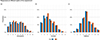 |
Figure 4. Histograms showing the distributions of (a) Annoyance, (b) Arousal, and (c) Valence responses to ASHP noise across Part 1 and Part 2 of the experiment. |
3.2 Subjective response to operating conditions and dynamic cycles
A key objective of this study was to explore people’s subjective reactions to different ASHP operating conditions. The three Operating Conditions (OC) considered in this study are Minimum Capacity (Defrost), Moderate Capacity, and Maximum Capacity. Figure 5 provides a histogram depicting the distribution of Annoyance, Arousal and Valence levels across three OCs in Part One of the experiment. The most noticeable differences in participants’ perceptions of ASHP noise are between the Minimum (Defrost) condition and the Moderate and Maximum capacities, while there seems to be a very slight difference between Moderate and Maximum capacities in general.
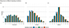 |
Figure 5. Histogram showing the distribution of (a) Annoyance, (b) Arousal and (c) Valence responses across different ASHP operating conditions in Part One of the experiment. |
Before conducting an in-depth analysis on how human response is influenced by the interaction between OCs, ASHP sound level, and Background Noise (BN) Level, a Friedman test is used to examine if participants’ responses during the Control condition are different from the other three OCs. This test indicated statistically significant differences among all variables (Annoyance, χ 2(3)=85.03, p < 0.001; Arousal, χ 2(3)=64.50, p < 0.001; and Valence, χ 2(3)=76.36, p < 0.001) across OCs. Post hoc Wilcoxon signed-rank tests (Bonferroni-adjusted) revealed that the Control condition differed significantly from all other conditions for Annoyance (p < 0.001 for all), Arousal (p < 0.001 for all), and Valence (p < 0.001 for all). Once it was established that responses were statistically significantly different, the Control condition was excluded from further analysis, as it did not contain any ASHP signal and was represented by only two stimuli in Part One.
A Linear Mixed Model (LMM) is used to assess how OCs, BN, and ASHP sound levels influence subjective response to ASHP noise. The LMMs with fixed effects for OC and interaction between BN and ASHP Sound Levels, and random intercepts for participants were fitted to account for the repeated measures design, participant-specific variability, and any unbalanced observations, thereby maximising the use of all available data. The Moderate capacity OC, with signals that include 31.5 dB(A) BN and 36.5 dB(A) ASHP Sound level, is used as the reference category (intercept). Visualisation of these interactions is presented in Figure 6, while the results of the statistical analysis are presented in Table 1.
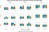 |
Figure 6. Subjective response as a function of operating condition (box colours), ASHP Sound Level (facets), and BN level (x-axis). Each boxplot shows the distribution of responses, with notches indicating median confidence intervals. Blue horizontal lines denote BN-level–specific mean ratings, and white points indicate overall means per operating condition. |
Results of Linear Mixed Models (LMMs) for subjective responses in Experiment Part 1 (Annoyance, Arousal, Valence) as a function of Operating Condition (OC), Background Noise (BN) level, ASHP Sound Level, and their interaction. The reference levels (intercept) were Moderate OC with 31.5 dB(A) BN and 36.5 dB(A) ASHP Sound Level.
The LMM for Annoyance (Tab. 1) yielded a marginal R 2 of 0.14 and a conditional R 2 of 0.73, indicating that fixed effects explained 14% of the variance while the full model (fixed + random effects) explained 73%.
Relative to the Moderate condition (intercept, M = 2.86, SE = 0.26), Annoyance was significantly lower in the Minimum condition (β = −0.36, SE = 0.06, t(2044)= − 5.49, p < 0.001), whereas there was no significant difference in Annoyance between the Moderate and Maximum conditions (β = −0.05, SE = 0.07, t(2043)= − 0.64, p = 0.525).
Annoyance increased significantly with higher ASHP Sound Levels. Compared to 36.5 dB(A), Annoyance was higher at 40 dB(A) (β = 0.84, SE = 0.09, t(2044.96)=8.93, p < 0.001) and substantially higher at 46 dB(A) (β = 2.31, SE = 0.09, t(2043.82)=24.94, p < 0.001). Similarly, higher BN (39.5 dB(A)) was associated with an increase in Annoyance (β = 0.56, SE = 0.09, t(2043)=6.04, p < 0.001).
However, significant interaction effects indicate that the impact of ASHP Sound Level depends on the BN level. At 39.5 dB(A) background, the increase in Annoyance typically associated with higher ASHP sound levels was attenuated. Specifically, the interaction between BN at 39.5 dB(A) and ASHP sound level at 40 dB(A) was negative (β = −0.54, SE = 0.13, t(2045.17)= − 4.09, p < 0.001), as was the interaction at 46 dB(A) ASHP level (β = −0.65, SE = 0.13, t(2043.07)= − 4.96, p < 0.001). These interactions suggest that increasing BN levels mitigated the increase in Annoyance caused by louder ASHP signals.
The LMM for Arousal (Tab. 1) converged at REML = 5989.9, with a random intercept variance of σ 2 = 1.693 (SD = 1.301) and residual variance σ 2 = 0.908 (SD = 0.953), revealing significant main effects of BN level, ASHP Sound Level, and OC. The marginal R 2 was 0.12, and the conditional R 2 was 0.70, indicating that most variance was explained by the combination of fixed and random effects.
Compared to the intercept (Moderate OC, BN 31.5 dB(A), ASHP 36.5 dB(A)), higher BN Levels (39.5 dB(A)) were associated with increased Arousal (β = 0.365, p < 0.001). Both ASHP 40 dB(A) and ASHP 46 dB(A) conditions yielded higher Arousal ratings (β = 0.475, p < 0.001; β = 1.617, p < 0.001, respectively). The Minimum OC was associated with reduced Arousal (β = −0.230, p < 0.001), while the Maximum OC did not differ significantly from the Moderate OC.
The LMM for Valence (Tab. 1) converged at REML = 5917.0, with a random intercept variance of σ 2 = 1.702 (SD = 1.304) and residual variance σ 2 = 0.873 (SD = 0.935), yielding a marginal R 2 of 0.13 and a conditional R 2 of 0.70. Compared to the intercept, higher BN level (39.5 dB(A)) was associated with reduced Valence (β = −0.368, p < 0.001). Both ASHP 40 dB and ASHP 46 dB conditions resulted in lower Valence ratings (β = −0.600, p < 0.001; β = −1.661, p < 0.001, respectively). The Minimum OC was associated with higher Valence (β = 0.240, p < 0.001), while the Maximum OC did not differ significantly from the Moderate OC.
Significant interaction effects indicated that the negative association between ASHP Sound Level and Valence was weaker under the higher BN level (39.5 dB(A)). Specifically, the reduction in Valence associated with ASHP 40 dB(A) (β = 0.329 (p = 0.001)) and 46 dB(A) (β = 0.447 (p < 0.001)) was less pronounced in this condition.
In Part Two, additional aspects of the ASHP conditions are considered, with particular focus on the potential impact of transitions between operating modes. The study examined two primary transition types, referred to as the “dynamic cycles”: transitions from Minimum to Maximum Capacity (Min-to-Max) and from Maximum to Minimum Capacity (Max-to-Min). In addition to the dynamic cycles, a continuous operating condition (“Stationary”) was included for comparison, along with a single Control condition without any ASHP sound emissions. However, for statistical purposes, the Control condition is not included in the LMMs.
In addition to dynamic cycles, LMM analysis for Part Two also included responses to two different time points (Transition and End), allowing assessment of whether responses vary across dynamic cycles and between the Transition and End time points. In these analyses, the Stationary condition with the End time point served as the reference category, providing a baseline against which both dynamic cycles and time points were compared. Results of this analysis can be seen in Table 2.
Results of Linear Mixed Models (LMMs) for subjective responses in Experiment Part 2 (Annoyance, Arousal, Valence).
The LMM for Annoyance converged at REML = 5665, with a random intercept variance of σ 2 = 3.050 (SD = 1.746) and residual variance σ 2 = 2.023 (SD = 1.422). The model yielded a marginal R 2 of 0.023 and a conditional R 2 of 0.611. This substantial difference between marginal and conditional R 2 show that while the model works well when accounting for individual differences, its ability generalise based on fixed effects alone is limited. Compared to the intercept (Stationary), both dynamic cycles were associated with significantly higher Annoyance ratings: β = 0.518, SE = 0.098, t(1490.19)=5.284, p < 0.001 for Max-to-Min, and β = 0.959, SE = 0.101, t(1490.23)=9.495, p < 0.001 for Min-to-Max. The Min-to-Max transition elicited the highest Annoyance scores among the dynamic cycles. In contrast, the difference in responses given at different time points (Transition vs. End) did not reach statistical significance (β = −0.037, p = 0.608), suggesting that Annoyance ratings were not reliably different at these two time points.
The LMM for Arousal ( ,
,  ) converged at REML = 4856.1, with a random intercept variance of σ
2 = 1.631 (SD = 1.277) and residual variance σ
2 = 1.200 (SD = 1.095). Relative to the intercept, both dynamic cycles produced significantly higher Arousal ratings: β = 0.326, SE = 0.076, t(1490.19)=4.319, p < 0.001 for Max-to-Min, and β = 0.681, SE = 0.078, t(1490.23)=8.747, p < 0.001 for Min-to-Max. As with Annoyance, the Min-to-Max transition elicited the highest Arousal responses. The responses given at two time points was not statistically significant (β = −0.032, p = 0.566).
) converged at REML = 4856.1, with a random intercept variance of σ
2 = 1.631 (SD = 1.277) and residual variance σ
2 = 1.200 (SD = 1.095). Relative to the intercept, both dynamic cycles produced significantly higher Arousal ratings: β = 0.326, SE = 0.076, t(1490.19)=4.319, p < 0.001 for Max-to-Min, and β = 0.681, SE = 0.078, t(1490.23)=8.747, p < 0.001 for Min-to-Max. As with Annoyance, the Min-to-Max transition elicited the highest Arousal responses. The responses given at two time points was not statistically significant (β = −0.032, p = 0.566).
Lastly, the LMM for Valence ( ,
,  ) converged at REML = 4946.4, with a random intercept variance of σ
2 = 1.455 (SD = 1.206) and residual variance σ
2 = 1.279 (SD = 1.131). Relative to the intercept, both dynamic cycles were associated with significantly lower Valence ratings: β = −0.394, SE = 0.078, t(1490.22)= − 5.047, p < 0.001 for Max-to-Min, and β = −0.660, SE = 0.080, t(1490.27)= − 8.213, p < 0.001 for Min-to-Max. The Min-to-Max transition produced the largest decrease in Valence. Similar to the previous results, Valence responses given at two time points were also not statistically significantly different from each other (β = 0.040, p = 0.482).
) converged at REML = 4946.4, with a random intercept variance of σ
2 = 1.455 (SD = 1.206) and residual variance σ
2 = 1.279 (SD = 1.131). Relative to the intercept, both dynamic cycles were associated with significantly lower Valence ratings: β = −0.394, SE = 0.078, t(1490.22)= − 5.047, p < 0.001 for Max-to-Min, and β = −0.660, SE = 0.080, t(1490.27)= − 8.213, p < 0.001 for Min-to-Max. The Min-to-Max transition produced the largest decrease in Valence. Similar to the previous results, Valence responses given at two time points were also not statistically significantly different from each other (β = 0.040, p = 0.482).
3.3 Comparison of subjective responses at two time points following operating transitions
In Part Two of the experiment, participants evaluated ASHP noise at two key moments: 10 s after a transition in operating conditions (Transition) and at the end of the recording (End), evaluating the entire sound recording. In addition to the analysis reported in the previous section (Tab. 2), further statistical analysis is conducted to understand if transitions in operating conditions affect subjective response. The Shapiro–Wilk Test revealed that the distributions of Annoyance, Arousal and Valence responses at both the Transition and End time points significantly deviated from normality (p < 0.0001 for all variables). As a result, the non-parametric Wilcoxon signed-rank test was used to compare the responses between these two points.
The analysis revealed no statistically significant differences between Transition and End responses for Valence (W = 108 514.5, p = 0.613), Arousal (W = 97 283, p = 0.744), or Annoyance (W = 114 777, p = 0.555). These findings are open to interpretation. One possibility is that the transition dominated the overall perception, shaping the responses to the entire recording. Alternatively, participants’ reactions remained unaffected by the transition. It is worth noting that the experiment featured the most extreme transitions–from minimum (defrost) to maximum capacity and vice versa. This suggests that transitions between less extreme operating conditions (e.g., from minimum to moderate capacity) are even less likely to provoke a strong reaction. Although responses to dynamic cycles and Stationary conditions were (statistically) significantly different, the lack of difference between Transition and End responses, also supported by the LMM analysis (Tab. 2), indicates that the perception of transition dominates overall impressions.
3.4 Impact of background noise towards ASHP noise perception
One of the critical research questions of this study was regarding the effect of Background Noise (BN) on the perception of ASHP noise. Data gathered from Part One of the experiment is used to answer this research question, as Part Two only included nighttime BN.
Figure 7 presents Annoyance, Arousal, and Valence responses as a function of the combined A-weighted sound pressure levels (LAeq, 20 s) of ASHP and background noise (BN), measured at the listener’s position. Stimuli with the lower background noise level (31.5 dB(A)) include ASHP levels starting below 30 dB(A), whereas those with the 39.5 dB(A) background begin at approximately 32 dB(A), resulting in a slightly different ASHP level range across background conditions. Interpretation, therefore, focuses on the overlapping ASHP range (approximately 32–40 dB(A)), where comparisons between background conditions are most robust.
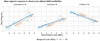 |
Figure 7. Mean subjective responses ((a) Annoyance, (b) Arousal, and (c) Valence) as a function of combined ASHP and BN sound pressure levels at the listener’s position, shown separately for BN levels of 31.5 dB(A) and 39.5 dB(A). Points indicate mean responses at each sound level; lines show linear trend fits. Responses were rated on different scales (Annoyance: 0–10; Valence and Arousal: 1–9) but are plotted on a common y-axis for alignment, and are restricted to the range covering the observed data for clarity. |
Linear trend lines are used to illustrate the overall direction of change in subjective responses as the sound level increases. Across this range, Valence decreases with increasing combined sound level, while Annoyance and Arousal increase. Additionally, it can be observed that the separation between the trendlines representing the two BN conditions tends to decrease with the increased SPL. This suggests that differences associated with background noise level become less pronounced as ASHP sound levels increase. This pattern is consistent with a reduced relative influence of background noise at higher ASHP levels; however, this observation is descriptive and is formally examined through statistical modelling.
Further statistical tests are conducted to examine the relationship between subjective response as a function of source distance and BN levels. Levene’s Homogeneity of Variance tests showed that the assumption of equal variance is violated for the three variables (Annoyance: F(7, 2015)=4.7881, p < 0.001; Arousal: F(7, 2015)=7.8528, p < 0.001; Valence: F(7, 2015)=3.4906, p < 0.001).
The Kruskal–Wallis test revealed a statistically significant difference in Annoyance responses, between stimulus combinations (χ
2(7)=329.58, p < 0.001), with an effect size of  . The Dunn’s test results between ASHP noise and Background Noise (BN) combinations (Tab. 3) reveal distinct patterns in how ASHP noise impacts Annoyance perception.
Dunn’s Test Z-statistics (top rows) and Bonferroni-adjusted p-values (bottom rows) for Annoyance responses across different ASHP and Background Noise (BN) LAeq, 20 s combinations.
The perception of Annoyance is more pronounced at higher ASHP sound levels. At lower BN levels (31.5 dB(A)), no significant differences are observed for 36.5 dB(A) ASHP noise compared to control conditions, indicating minimal impact. However, significant increases in Annoyance are observed at 40 dB(A) and 46 dB(A). At 46 dB(A), ASHP noise consistently dominates Annoyance perception, even when background noise is higher, suggesting a threshold effect. At higher BN levels (39.5 dB(A)), the masking effect of BN reduces the Annoyance perception at lower ASHP levels (36.5 dB(A) and 40 dB(A)), but higher ASHP sound levels (46 dB(A)) still trigger significant Annoyance. These findings suggest that higher ASHP sound levels consistently elicit Annoyance, regardless of BN, while lower ASHP levels are more likely to be masked by higher BN.
For the Arousal responses, the Kruskal–Wallis test showed statistically significant differences across ASHP and BN combinations (χ
2(7)=229.62, p < 0.001), with an effect size of  . Dunn’s test is used to further examine differences in Arousal responses across ASHP–BN combinations (Tab. 4).
Dunn’s Test Z-statistics (top rows) and Bonferroni-adjusted p-values (bottom rows) for Arousal responses across different ASHP and Background Noise (BN) LAeq, 20 s combinations.
As shown in Table 4, Arousal responses are influenced more by changes in ASHP sound levels than by BN levels alone. At lower background levels (31.5 dB(A)), significant differences emerge at 40 dB(A) ASHP noise and above. At higher background levels (39.5 dB(A)), a masking effect is observed, where responses to ASHP noise are similar to those for the background noise, except at 46 dB(A), where ASHP noise dominates. These results show that higher ASHP sound levels consistently lead to greater Arousal, with the largest differences at 46 dB(A). This suggests that higher BN levels reduce the perceptual differences between ASHP and ambient sounds, moderating Arousal responses up to a threshold.
For Valence, the Kruskal–Wallis test revealed statistically significant differences across the ASHP noise and BN level combinations (χ
2(7)=326.15, p < 0.001), with an effect size of  , indicating a large effect and meaningful difference between groups. The post hoc analysis using Dunn’s test suggests that ASHP sound levels and BN levels influence human response. Table 5 shows that Valence responses decrease as ASHP sound levels increase. At lower BN levels (31.5 dB(A)), 36.5 dB(A) ASHP noise does not significantly differ from control conditions, but at 40 dB(A) and 46 dB(A) ASHP noise, responses become significantly more negative. At higher BN levels (39.5 dB(A)), 36.5 dB(A) ASHP noise has a reduced impact, with responses similar to the 39.5 dB(A) control, suggesting a masking effect.
Dunn’s Test Z-statistics (top rows) and Bonferroni-adjusted p-values (bottom rows) for Valence responses across different ASHP and Background Noise (BN) LAeq, 20 s combinations.
These findings align with the subjective response trends shown in Figure 7. Annoyance increases with increasing ASHP sound level under both background noise conditions, while Arousal shows a similar increasing tendency. In contrast, Valence decreases with increasing ASHP sound level, indicating a more negative perceptual response at higher levels. A more detailed explanation of the patterns observed in Tables 3–5 is provided in Appendix A.
The lack of significant differences between the two background noise levels (31.5 dB(A) vs. 39.5 dB(A)) is likely due to the nature of the control stimuli, which consisted of filtered pink noise with no salient or memorable content. As participants were not directly comparing these control conditions and were exposed to numerous acoustically varied ASHP stimuli in between, it is plausible that level differences in otherwise featureless signals did not result in distinguishable or memorable perceptual effects.
3.5 Influence of ownership
To understand whether the participants responded more favourably to the sound of their own heat pump than to a heat pump of unknown ownership, they were presented with one of two scenarios. In Scenario 1, participants were informed that the ASHP belonged to them, while in Scenario 2, no ownership information was provided.
The results of a Shapiro–Wilk Normality Test indicated that the responses were not normally distributed for any of the three metrics: Valence (Scenario 1: W = 0.96, p < 0.001; Scenario 2: W = 0.96, p < 0.001), Arousal (Scenario 1: W = 0.93, p < 0.001; Scenario 2: W = 0.93, p < 0.001), and Annoyance (Scenario 1: W = 0.95, p < 0.001; Scenario 2: W = 0.96, p < 0.001). Therefore, the Mann–Whitney U Test was used to compare the distributions of these variables across scenarios.
Among the three response variables, only Annoyance differed significantly between ownership conditions (W = 1 701 181, p < 0.001). Mean Annoyance was slightly lower in Scenario 1 (Participant owns the ASHP) (M = 3.62, SD = 2.35) than in Scenario 2 (No ownership information) (M = 3.91, SD = 2.28), corresponding to a mean difference of −0.29 on the 9-point scale. Median Annoyance ratings were identical across scenarios (median = 4), and the associated effect size was small (r = −0.06), indicating a modest distributional shift rather than a pronounced separation between groups.
No statistically significant differences were observed for Valence (Scenario 1: M = 5.17, SD = 1.78; Scenario 2: M = 5.00, SD = 1.66; W = 1 887 728, p = 0.053, r = 0.03) or Arousal (Scenario 1: M = 3.46, SD = 1.86; Scenario 2: M = 3.45, SD = 1.56; W = 1 803 712, p = 0.607, r = −0.01). Median values for both variables were identical across scenarios.
As illustrated in Figure 8, Annoyance distributions overlap substantially between ownership conditions, consistent with the small effect size observed. The statistically significant result for Annoyance, therefore, reflects the large sample size and the sensitivity of rank-based tests to small but systematic shifts in the response distribution. Overall, these findings suggest that perceived ownership of the ASHP may slightly reduce reported Annoyance; however, the practical impact of this effect appears limited, and ownership should be interpreted as a contextual modifier rather than a primary determinant of perception of ASHP noise. It is worth noting that the ownership manipulation may also influence the distributional characteristics of Annoyance ratings in the full dataset. For example, the divergence in responses between ownership and non-ownership groups could lead to bimodal patterns or increased variability, which may affect subsequent analyses if not explicitly accounted for. Further studies could explore this interaction in greater detail.
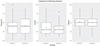 |
Figure 8. Comparison of Annoyance, Arousal and Valence responses across ownership scenarios (Scenario 1 = ASHP belonged to the participant, Scenario 2 = No information was provided). Red dots indicate the mean values. |
3.6 Subjective response and sound quality metrics
The relationships between participants’ subjective evaluations (Annoyance, Arousal, Valence) and Sound Quality Metrics (SQM) were examined using Spearman’s ρ correlation analysis. The results reflect the acoustic character of ASHP noise and A-weighted sound pressure levels of the ASHPs (LAeq, 20 s and LAeq, 60 s), as shown in Table 6. BN levels are excluded from this analysis, as only Part One included both BN conditions.
Spearman’s ρ correlation coefficients between subjective response variables (Annoyance, Arousal, Valence) and Sound Quality Metrics (SQMs), including ASHP sound levels.
Responses to the stimuli from Part One and Part Two follow the same trends and show no significant deviation from the overall correlation coefficients calculated across both parts. The only exception is Sharpness, which exhibits weak correlations in Part Two (r < 0.3 across all variables), but shows most values to be moderate correlations in Part One (r ranging from −0.289 to −0.315), only one falling below the lower bound of the moderate range.
While all correlations between all pairs reached statistical significance, the correlation coefficients between Fluctuation Strength and all three subjective response variables were notably low. In the overall dataset, there were statistically significant moderate correlations between Annoyance and Loudness (r(3518)=0.388, p < 0.001), Partial Loudness (r(3518)=0.328, p < 0.001), Roughness (r(3518)=0.366, p < 0.001), and Tonality (r(3518)=0.305, p < 0.001). A statistically significant negative correlation was also observed between Annoyance and Sharpness (r(3518)= − 0.293, p < 0.001), falling just below the conventional threshold for a moderate association.
Arousal exhibited a moderate positive correlation with Loudness (r(3518)=0.359, p < 0.01), Roughness (r(3518)=0.332, p < 0.01), Tonality (r(3518)=0.323, p < 0.01), and a low positive correlation with Partial Loudness (r(3518)=0.290, p < 0.01), while showing a low negative correlation with Sharpness (r(3518)= − 0.259, p < 0.01).
In contrast to the predominantly positive associations observed for Annoyance and Arousal, the SQMs, apart from Sharpness, were negatively correlated with Valence. Valence responses showed a moderate negative correlation with Loudness (r(3518)= − 0.381, p < 0.01), Roughness (r(3518)= − 0.367, p < 0.01), and Partial Loudness (r(3518)= − 0.333, p < 0.01), a low negative correlation with Tonality (r(3518)= − 0.298, p < 0.01), and a low positive association with Sharpness (r(3518)=0.296, p < 0.01). It should be noted that for the Valence responses in Part One, Partial Loudness showed an association almost as strong as standard Loudness.
Finally, the correlations between ASHP SPL (LAeq, 20 s and LAeq, 60 s) and the subjective response variables (Annoyance, Arousal and Valence) suggested trends similar to those observed between ASHP and BN combinations and subjective response in Figure 7. Valence has a moderate negative association with ASHP sound levels (r(3518)= − 0.361, p < 0.01), suggesting that higher ASHP sound levels were perceived as less pleasant. Both Arousal (r(3518)=0.323, p < 0.01) and Annoyance (r(3518)=0.359, p < 0.01) had statistically significant positive associations with ASHP sound levels, indicating that as the noise levels from the heat pump increased, it became more annoying and stimulating.
Among all the SQMs, Loudness is shown to have the strongest association with the subjective response variables. Roughness ranked second, which showed almost similar, and in some cases, the highest correlation coefficients relative to ASHP sound levels. Partial Loudness and Tonality followed these, which showed a statistically significant low to moderate association between subjective responses. Two of these significant SQM variables showed higher or comparable correlations with subjective response than sound levels. These findings suggest that the acoustic character of ASHPs significantly affects human perception and needs to be considered in the planning process.
A Generalised Linear Mixed Model (GLMM) with a Beta distribution and logit-link function was applied to model the impact of SQM on Annoyance, Arousal and Valence (Tab. 7). In this model, Loudness, Tonality, and Roughness were considered fixed effects and significant predictors across all three response variables. In contrast, Sharpness and Fluctuation were not statistically significant in any models and were not considered among fixed effects.
GLMMs were fitted with a random intercept for participants and a random slope for Loudness. This structure allowed the model to account for individual differences in overall response levels and to let the effect of Loudness vary across participants. Inclusion of random intercepts for Loudness was justified, given that it showed the highest associations with subjective responses in the Spearman correlation analysis (Tab. 6). The equation corresponding to the GLMM model is:
 (1)
(1)
Where:
-
Y ∈ (0, 1) represents the scaled response variables (Annoyance, Arousal, Valence).
-
i denotes the observation index, and j denotes the participant index.
-
μij is the expected value of the response variable for observation i from participant j.
-
ϕ is the precision parameter of the Beta distribution.
-
The fixed effects include β0 (intercept), β1, β2, and β3, representing the coefficients for Loudness, Tonality, and Roughness, respectively.
-
The random effects comprise u0j ∼ 𝒩(0, σu0 2), the random intercept for participant j, and u1j ∼ 𝒩(0, σu1 2), the random slope for Loudness for participant j.
-
The logit-link function ensures that predicted values remain within the bounded interval (0, 1), appropriate for the Beta distribution.
Additional exploratory models, including individual noise sensitivity scores (NoiseQ) as a fixed effect, were fitted. However, in all three outcomes, NoiseQ did not produce statistically significant effects (Annoyance GLMM: p = 0.0278; Valence GLMM: p = 0.382; Arousal GLMM: p = 0.254) and did not improve the fit of the model. Therefore, NoiseQ was not retained in the final models.
The variable SPL (LAeq, 20 s and LAeq, 60 s) was not included among the fixed effects in the final model. During the model development phase, multicollinearity was observed between ASHP SPL and Loudness when both variables were included. Models that included only loudness performed equally or better than those that included ASHP SPL. Given the aim of creating a model addressing the acoustic character of ASHPs, models with Loudness were preferred over those with ASHP SPL.
In the Annoyance model, the adjusted Intraclass Correlation Coefficient (ICC) was 0.921, indicating that individual differences account for a substantial portion of variance in Annoyance responses. Each fixed effect was a statistically significant positive predictor, meaning that increases in these psychoacoustic metrics are associated with increased Annoyance. VIF values were low (1.15–1.32), indicating minimal multicollinearity. Ten-fold cross-validation yielded an Root Mean Square Error (RMSE) of 1.204, R 2 of 0.733, and Mean Absolute Error (MAE) of 0.895, demonstrating that the model generalises reasonably well to unseen data while highlighting the dominant contribution of random effects.
In the Arousal model, the adjusted ICC was 0.799, confirming that a dominant portion of response variance is attributable to between-participant differences. The fixed effects of Loudness, Tonality, and Roughness were all statistically significant predictors of Arousal, with positive coefficients indicating that increases in these psychoacoustic metrics increase Arousal. VIF values were within acceptable ranges, indicating minimal multicollinearity. Cross-validation results showed an RMSE of 0.951, R 2 of 0.690, and MAE of 0.712. These results demonstrate that the model generalises well to unseen data, though the high ICC highlights that individual variability remains the primary driver of response magnitude.
In the Valence model, the adjusted ICC was 0.907, suggesting that a very large proportion of the variance in Valence ratings is attributable to between-participant variability rather than fixed effects alone. All fixed effects were statistically significant and contributed negatively to the model, indicating that increases in these values decrease Valence. The Variance Inflation Factor (VIF) values were below the typical threshold of 5, suggesting minimal multicollinearity. Additionally, 10-fold cross-validation yielded an RMSE of 0.958, an R 2 value of 0.681, and an MAE of 0.695. While the marginal R 2 value is relatively low (0.157), the high conditional R 2 (Tab. 7) and cross-validation scores confirm that the model predicts responses accurately when accounting for individual differences.
The GLMM analysis showed that Loudness, Tonality, and Roughness are the primary psychoacoustic predictors of Annoyance, Arousal, and Valence, consistently outperforming SPL in model fit. While increased Loudness, Tonality, and Roughness characteristics result in significantly increased Annoyance and Arousal and decreased Valence, NoiSeQ did not emerge as a significant predictor. Additionally, ICC values across all models highlight that a substantial portion of the variance in human perception of ASHP noise is driven by individual differences rather than acoustic character alone.
4 Discussion
The results of the study revealed that Annoyance, Arousal and Valence responses to ASHP noise emissions are affected by changes in the operating condition. However, further analysis (Tab. 2) showed that the differences in subjective response are affected by major changes in the ASHP operation (i.e., changes from Minimum to Maximum) and not affected by changes from Medium to Maximum capacity conditions.
Moreover, the findings demonstrate that sound quality metrics, such as Loudness, Tonality, and Roughness, significantly influence subjective responses to ASHP noise and may capture perceptual impacts that A-weighted SPL alone does not. Spearman’s correlation analysis (Tab. 6) supports this empirically: Loudness and Roughness exhibit equally important or almost as strong associations with subjective responses (Annoyance, Arousal, and Valence) as LAeq-based metrics, with Tonality also showing meaningful correlations. These results align with prior studies (e.g. [10]) that have argued for including spectral and temporal features in assessments of heat pump noise.
These empirical findings underline the perceptual salience of specific acoustic features, which, in turn, raise broader questions about the adequacy of current regulatory frameworks, such as for the existing UK guidelines, ASHP sound pressure levels are required not to exceed 37 dB(A) when measured one meter away from the window of nearest habitable room of a neighbouring property. In quieter residential contexts, such as rural areas, even planning compliant ASHP noise may exceed perceptual thresholds, leading to heightened annoyance. In contrast, in noisier urban environments, masking effects from background activity may reduce the perceptual prominence of such features, though this should not be misinterpreted as justification for relaxed protections. Rather, this calls for a context-sensitive approach to regulation, one that incorporates perceptual data and accounts for how individuals experience sound in situ, in line with the soundscape approach outlined in ISO 12913 [40]. Regulation guided by both physical metrics and lived experience can help ensure that protection from noise is distributed more equitably, regardless of baseline environmental sound levels.
Recent research carried out by Goecke et al. [41] used noise emissions from a heat pump as an application example to show how psychoacoustic mapping can be used to predict sound emissions to contribute to modern urban development. In addition to using the A-weighted sound levels, the psychoacoustic mapping prepared using SoundPLANnoise [42] maps the propagation of Loudness and Sharpness, with mapping of Tonality under development. The propagation of psychoacoustic quantities of sound can be different from sound pressure. Sharpness, for example, decreases less with distance compared to Loudness or sound pressure level [41]. Even though the sound emissions from an ASHP are within the limits, it can still lead to annoyance at traditionally unexpected distances. Along with the psychoacoustic findings presented in this paper, this suggests that corrections for the acoustic character of the heat pumps must be further considered to reduce the noise impacts of sustainable technologies like ASHPs and facilitate broader acceptance.
The model fit metrics of the GLMM model, presented in Table 7, show substantial differences between the Marginal R2 (Rm2) and Conditional R2 (Rc2) values. Note that these parameters represent the explanatory power of the full model, whereas Cross-Validation metrics (RMSE, MAE) assess predictive generalisability. In the Annoyance model, where Rm2 = 0.161 and Rc2 = 0.934, the outcome suggests that while the fixed effects (psychoacoustic metrics) explain a moderate portion of the variance, the model captures a very high degree of within-sample variability when individual differences are accounted for. This highlights that the variability in Annoyance responses is largely attributable to participant-specific factors. Additionally, a similar pattern between Rm2 and Rc2 is observed in the LMM analyses reported in Tables 1 and 2, confirming that a substantial portion of variance is driven by participant-level differences not captured by fixed effects alone.
GLMMs for Annoyance, Arousal, and Valence (Beta Distribution with Random Slopes). For each model, the Akaike Information Criterion (AIC) value, the marginal coefficient of determination (Rm 2), the conditional coefficient of determination (Rc 2), and regression estimates are reported. ICC refers to the Adjusted Intraclass Correlation Coefficient. VIF refers to Variance Inflation Factor.
The GLMM model explicitly modelled this variability through random effects. Crucially, the inclusion of a random slope for Loudness indicates that individuals differ not only in their baseline annoyance levels but also in their sensitivity to changes in Loudness. This suggests that some individuals may be highly reactive to loudness increases, while others are more tolerant. The statistically significant but very weak correlations between the NoiseQ and subjective responses indicate that this individual variability cannot be fully attributed to self-reported noise sensitivity. Moreover, findings confirm that Loudness, Tonality, and Roughness significantly influence Annoyance responses to ASHP noise, with notable inter-individual variation. If regulatory frameworks consider such models, they must balance predictive accuracy with simplicity. Loudness emerged as the strongest and most consistent predictor across conditions, suggesting it can potentially complement SPL in standards. However, A-weighted SPL remains necessary for compatibility with existing regulations. Future work should explore hybrid models combining SPL and Loudness to provide a simple, robust implementation that optimises the cost-benefit ratio.
The results of this study reveal significant patterns in how varying ASHP sound levels, in relation to BN, influence human emotional responses, particularly Annoyance. Statistical analysis shows that ASHP sound levels above 40 dB(A) consistently trigger higher Annoyance, for the BN conditions we consider. In contrast, lower ASHP sound levels are more susceptible to masking by background noise. At the highest ASHP noise level (46 dB(A)), background noise fails to mask the impact on Annoyance, while lower ASHP sound levels are more easily masked.
This finding for BN is consistent with the complex role of masking in environmental acoustics. Along with established A-weighted sound levels and SQMs, Partial Loudness was considered in this analysis to account for how ambient background noise affects the perception of ASHP signals. The Moore–Glasberg Partial Loudness model [38] successfully accounted for the contribution of BN, yielding statistically significant low-to-moderate associations with subjective responses across all parts. Although standard Loudness exhibited stronger correlations within this specific dataset, incorporating Partial Loudness offers a valuable framework for future research. This is especially evident when Partial Loudness’s performance in Valence responses is compared to standard Loudness in Part One (Loudness (r(3518)= − 0.348), Partial Loudness (r(3518)= − 0.338)). Given the operational differences between the stimuli where Part One involved continuous ASHP operation, while Part Two featured transient signals, the model successfully captures the steady-state masking of continuous ASHP noise by the ambient background. Because this steady-state masking effectively smooths out the intrusive features of the continuous signal, it directly mitigates perceived harshness, which maps closely onto the pleasantness-unpleasantness dimension of Valence. On the other hand, temporal fluctuations and swift envelope changes that are currently more heavily weighted by standard Loudness may be introduced by the dynamic nature of the transient operations in Part Two. Specifically, Partial Loudness can be utilised to establish more precise masking thresholds, aiding in the assessment and optimisation of ASHP noise limits across diverse ambient environments.
As an alternative to the Moore–Glasberg approach, the Sottek Hearing Model, which was used to calculate the perceptual quantities of Tonality, Roughness, and Fluctuation Strength [37] in this study, is currently being extended to encompass partial sound qualities, including Partial Loudness. As the official, validated implementation of this extended Sottek framework undergoes final experimental verification, it will provide a valuable alternative for precise quantification of the ASHP signal’s prominence relative to varying BN thresholds in the future studies.
These observations regarding BN have important implications for the future regulation of ASHP noise, particularly in residential settings, where community acceptance is critical. This study highlights the need to focus on the effect of background noise. Global policies must account for the interaction between ASHP noise characteristics and varying background noise levels. As a result, this oversight could lead to discrepancies between regulatory limits and actual human perception of noise annoyance.
Considering these findings, policies regarding ASHP noise could benefit from a more dynamic regulation approach that accounts for variations in background noise and psychoacoustic characteristics. In particular, ASHPs could be subject to stricter noise regulations in rural areas where the background noise is lower and psychoacoustic effects, like Tonality, are more pronounced. In contrast, more flexible criteria could be applied in urban environments where higher background noise levels could mask the ASHP noise to a degree. Such an approach would help reduce the likelihood of unnecessary denials of planning applications in urban areas while protecting the residents in quieter, rural environments from potentially disruptive ASHP noise.
This study focused on human responses to noise emissions from a single ASHP. However, there is growing concern about the cumulative impacts of multiple ASHPs operating in the same area. Currently, the cumulative effect of ASHPs is not well known, and there is a lack of understanding of how communities newly exposed to multiple ASHPs would respond to it. The noise regulations are not yet designed to account for the effects of multiple units. For example, in the UK, ASHPs installed under PDR are not subject to assessments that adequately account for cumulative noise impacts [9]. This could adversely affect residents’ wellbeing and slow down wider adoption if they remain unaccounted for. To address this gap, future studies should prioritise investigating the cumulative impact of multiple ASHPs, particularly in residential areas where such installations are becoming more common and particularly in multi-family buildings or high density contexts.
When interpreting the findings of this study, it is important to consider that certain methodological decisions were taken to reflect the worst-case scenarios. Firstly, the study employed two representative ASHP recordings selected to capture a meaningful range of psychoacoustic characteristics. The microphone position was deliberately chosen based on the angle of maximum noise emission to reflect a worst-case exposure scenario. While this approach does not capture full spatial directivity or the entire diversity of ASHP models, it provides a robust and consistent basis for assessing perceptual responses. Future work will expand the range of ASHP types and incorporate directivity data to increase generalisability.
Secondly, although the background noise spectrum used in the experiment was based on the standardised Spectrum No. 2 from BS EN ISO 717-1:2020 [26], which represents typical road traffic noise in terms of one-third octave band composition, it does not replicate the full temporal, spatial, and semantic complexity of real-world environmental soundscapes. As such, differences in masking behaviour and subjective impressions may exist compared to actual outdoor acoustic conditions.
Lastly, this experiment considered a partially open window scenario to investigate a potential worst-case condition, which also reflects a plausible real-life situation. While ASHPs are commonly used for heating indoor spaces during winter, they are used year-round for domestic hot water production, which may also occur during nighttime. Laboratory studies have shown that even small openings (e.g. tilted windows) significantly increase the risk of sleep disruption due to ASHP noise emissions [23]. Future field studies should assess the long-term sleep impacts of ASHP noise, as well as the potential for low-frequency noise transmission through closed windows. Additionally, although it was not within the scope of this paper, ASHPs are also used for cooling residential spaces in warmer regions. This implies that ASHP noise may adversely affect neighbouring properties even during warm daytime conditions. Such impacts could significantly affect the quality of life in neighbouring dwellings that rely on natural ventilation in warm climates. Future research should compare the noise impact of ASHPs during cooling versus heating operation, examine how this compares to traditional mechanical cooling systems (e.g. air conditioning units), and investigate how such noise is perceived by affected residents.
5 Conclusions
This study investigated how background noise levels, operating conditions, and the acoustic characteristics of ASHP noise affect human subjective responses. Participants’ responses to Continuous vs. Variable operation were analysed across different operating conditions, background noise levels, A-weighted sound pressure levels, and Sound Quality Metrics (SQM). Specifically, we considered participants’ Annoyance, Arousal, and Valence responses across these conditions. It was shown that Annoyance, Arousal, and Valence responses are significantly affected by A-weighted ASHP sound levels, with higher SPL correlating with increased Annoyance and Arousal and decreased Valence, as might be predicted.
One of the main aims was to understand the psychoacoustic characteristics of ASHP noise. SQMs, such as Loudness, Sharpness, Roughness, and Tonality, are low-to-moderately associated with subjective response to ASHP noise. Among these, Loudness consistently showed stronger correlations with subjective responses than A-weighted sound levels. Roughness, however, showed a stronger association than A-weighted levels only in the overall analysis and showed weaker associations with human response in the separate analyses of Parts 1 and 2. Tonality was the third most strongly associated metric, with correlation coefficients close to A-weighted levels in the overall analysis, but notably weaker in the part-specific analyses. The fact that these psychoacoustic metrics are more than or nearly as influential as A-weighted noise levels further emphasises the importance of acoustic characteristics, suggesting that tonal characteristics contribute meaningfully to perceived annoyance and overall sound perception. These results highlight the limitations of regulatory approaches that rely solely on A-weighted sound levels and point to the need to incorporate psychoacoustic factors into noise assessment and policy frameworks for ASHP installations. However, it is important to state that any amendment to the policy must consider streamlined means of regulating the ASHP installations while still prioritising people’s wellbeing. The homeowners or the installers should not be overburdened with unnecessary tasks or administration.
Another significant finding of the study was related to Background Noise levels (BN). Statistical analysis showed that the daytime BN levels, especially, can mask the lower ASHP A-weighted noise levels (lower than 40 dB(A)). When ASHP sound levels are above 40 dB(A), and especially at 46 dB(A), the masking effect associated with both background noise levels becomes largely reduced, leading to increased annoyance. Taken together, these findings indicate that the influence of background noise is most relevant at lower ASHP levels, where higher daytime background noise can partially mask ASHP emissions. Importantly, this does not imply that increases in ASHP noise are acceptable simply because an environment is already noisy. Rather, the results suggest that a single, fixed noise limit applied irrespective of background conditions and contextual factors may be overly restrictive at moderate ASHP levels. Instead, the results support the consideration of differentiated ASHP noise limits, with stricter thresholds during nighttime conditions and a modestly higher allowable limit during daytime periods, limited to the range where masking remains effective.
An interesting finding of the study concerned heat pump ownership. Participants responded more positively to the noise from an ASHP they were told was their own than to the noise of a unit of unknown ownership.
Lastly, the study considered the effect of continuous and variable ASHP noise. Subjective responses to Continuous operation (Part One) and Variable operation (Part Two) conditions followed similar patterns. Participants’ responses to the Minimum capacity condition (Defrost) were significantly more positive compared to the Maximum capacity condition. Responses elicited immediately after a transition in operational capacity were not statistically significantly different from the responses given to the overall signal. This may be primarily because the perception of transition dominates the overall response to the ASHP noise. However, the absence of statistically significant differences between immediate and overall responses to transitions may reflect the complexities of the perceptual changes involved. Future research should further look at how specific experimental design choices, such as timing, transition types, and participant attention, affect the sensitivity of such comparisons.
These findings suggest limitations in current regulatory frameworks, which rely primarily on SPL thresholds without considering the environmental factors or the acoustic character of the ASHP noise. Hence, psychoacoustic considerations and tailoring the noise assessment procedure to specific environmental contexts should be integrated into the regulations to improve wellbeing in domestic environments and facilitate the broader adoption of ASHPs.
Acknowledgments
We want to thank Christoph Reichl from the Austrian Institute of Technology and Christian Kasess from the Austrian Academy of Sciences for providing us with access to their Air Source Heat Pump recording datasets.
Funding
This study is conducted as part of the Future Homes Project funded under the Innovation Accelerator programme of Innovate UK (Project number 10054845).
Conflict of interest
The authors declare no conflicts of interest.
Data availability statement
Data are available on request from the authors.
References
- Natural Resources Canada: Heating and Cooling with a Heat Pump, 2009. URL https://natural-resources.canada.ca/energy-efficiency/energy-star-canada/about/energy-star-announcements/publications/heating-and-cooling-heat-pump/6817. Last Modified: 2022-08-09 publisher: Natural Resources Canada. [Google Scholar]
- M. Habibi, A. Hakkaki-Fard: Long-term energy and exergy analysis of heat pumps with different types of ground and air heat exchangers. International Journal of Refrigeration 100 (2019) 414–433. ISSN 01407007. [Google Scholar]
- European Commission: European Green Deal: Commission proposes to boost renovation and decarbonisation of buildings, 2021. URL https://ec.europa.eu/commission/presscorner/detail/en/ip_21_6683. [Online; accessed 2024-12-04]. [Google Scholar]
- Europe – Total CO2 emissions, 2022. URL https://www.iea.org/regions/europe/emissions. [Online; accessed 2025-05-14]. [Google Scholar]
- P. Carroll, M. Chesser, P. Lyons: Air source heat pumps field studies: a systematic literature review. Renewable and Sustainable Energy Reviews 134 (2020) 110275. ISSN 1364-0321. [Google Scholar]
- D. Peñaloza, É. Mata, N. Fransson, H. Fridén, Á. Samperio, A. Quijano, A. Cuneo: Social and market acceptance of photovoltaic panels and heat pumps in Europe: a literature review and survey. Renewable and Sustainable Energy Reviews 155 (2022) 111867. ISSN 13640321. [Google Scholar]
- M. Poblete-Cazenave, N.D. Rao: Social and contextual determinants of heat pump adoption in the US: implications for subsidy policy design. Energy Research & Social Science 104 (2023) 103255. ISSN 22146296. [Google Scholar]
- IEA: Europe annual heat pump sales, 2013-2023 – Charts – Data & Statistics, 2024. URL https://www.iea.org/data-and-statistics/charts/europe-annual-heat-pump-sales-2013-2023. [Online; accessed 2024-12-04]. [Google Scholar]
- DESNZ: Review of air source heat pump noise emissions, permitted development guidance and regulations. Technical Report, Department for Energy Security and Net Zero, 2024. [Google Scholar]
- M. Torjussen: Sound from domestic air source heat pumps: a case study, in: Proceedings of the Institute of Acoustics. Vol. 42. Institute of Acoustics, Milton Keynes, 2020. [Google Scholar]
- C. Reichl: IEA HPT Annex 51: acoustic signatures of heat pumps – Final report. Technical Report HPT-AN51-1, Heat Pump Centre, 2021. [Google Scholar]
- C. Reichl: IEA HPT Annex 63: placement impact on heat pump acoustics, 2023. URL https://heatpumpingtechnologies.org/annex63/. [Online; accessed 2024-12-05]. [Google Scholar]
- MCS 020 a) ISSUE 1.1 air source heat pump sound calculation (For permitted development installations), 2025. [Google Scholar]
- P. Brandstätt, M. Krämer, B. Kaltbeitzel: Noise and vibration characteristics of outdoor heat pumps, in: Proceedings of ICSV 30, Amsterdam, 2024. [Google Scholar]
- S. Wagner, X. Carniel, J. Rohlfing, K. Bay, H. Hellgren: 3: overview on heat pump component noise and noise control techniques. Technical Report, 2020. [Google Scholar]
- BSI: BS 4142:2014+A1:2019 | 30 Jun 2019 | BSI Knowledge, 2019. [Online; accessed 2024-10-08]. [Google Scholar]
- R. Fumagalli, P. Wagner, R. Pratter, R. Rieberer, F. Bessac, M. Mondot, H. Hellgren, A. Troll, P. Lachman: Acoustic signatures of heat pumps final report – Part 4 1.2 regulations – Countries overview. Technical Report, Heat Pump Centre, 2020. [Google Scholar]
- L. Stürenburg, H. Braren, L. Aspöck, J. Fels: Loudness and preference judgments for noises of a heat pump, in: INTER-NOISE and NOISE-CON Congress and Conference Proceedings. Vol. 270, 2024, pp. 5415–5423. ISSN 0736-2935. [Google Scholar]
- H. Hellgren, C.H. Kasess: IEA HPT Annex 51: acoustic signatures of heat pumps – Final report – Part 12 – 6 annoyance rating and psychoacoustical analysis of heat pump sound. Technical Report HPT-AN51-12, Heat Pump Centre, 2020. [Google Scholar]
- C.H. Kasess, C. Reichl, H. Waubke, P. Majdak: Perception rating of the acoustic emissions of heat pumps, in: Forum Acusticum, Lyon, France, 2020, pp. 2453–2458. [Online; accessed 2024-04-09]. [Google Scholar]
- World Health Organization (WHO) environmental noise guidelines for the european region. Technical Report, 2018. Container-title: Larmbekampfung. Vol. 13. ISSN: 18634672. [Google Scholar]
- M. Basner, W. Babisch, A. Davis, M. Brink, C. Clark, S. Janssen, S. Stansfeld: Auditory and non-auditory effects of noise on health. Lancet 383, 9925 (2014) 1325–1332. [CrossRef] [PubMed] [Google Scholar]
- S. Benz, D. Schreckenberg, B. Vassallo, M. Braun, C. Eulitz, T. Penzel, M. Glos, L. Alt, K. Lederer: Annoyance and sleep disturbance due to noise from air-source heat pumps and air conditioners. Technical Report 152/2024, German Environment Agency, 2024. [Google Scholar]
- Building Performance Centre, Edinbrugh Napier University: Ee0214 Acoustic Noise Measurements of Air Source Heat Pumps. Ee0214, 2011. [Google Scholar]
- C. Skinner, G. Colin: The National Noise Incidence Study 2000/2001 (United Kingdom): Volume 1 – Noise levels. Technical Report 206344f, BRE Environment, United Kingdom, 2000. [Google Scholar]
- BSI: BS EN ISO 717-1:2020 Acoustics. Rating of sound insulation in buildings and of building elements – Airborne sound insulation, 2020. [Google Scholar]
- A.J. Torija, I.H. Flindell: The subjective effect of low frequency content in road traffic noise. Journal of the Acoustical Society of America 137, 1 (2015) 189–198. ISSN 0001-4966, 1520-8524. [NASA ADS] [CrossRef] [Google Scholar]
- N. Zacharov, Ed.: Sensory Evaluation of Sound. CRC Press, 2018. ISBN 978-0-429-42942-2. [Google Scholar]
- T. Waters-Fuller, D. Lurcock: Nanr116: ‘Open/Closed window research’ sound insulation through ventilated domestic windows. Technical Report, The Building Performance Centre, School of the Built Environment, Napier University, 2007. [Google Scholar]
- M. Schütte, A. Marks, E. Wenning, B. Griefahn: The development of the noise sensitivity questionnaire. Noise & Health 9, 34 (2007) 15–24. ISSN 1463-1741. PMID: 17851223. [Google Scholar]
- M.M. Bradley, P.J. Lang: Measuring emotion: the self-assessment manikin and the semantic differential. Journal of Behavior Therapy and Experimental Psychiatry 25, 1 (1994) 49–59. ISSN 00057916. [CrossRef] [PubMed] [Google Scholar]
- J.A. Russell: A circumplex model of affect. Journal of Personality and Social Psychology 39, 6 (1980) 1161–1178. ISSN 1939-1315(Electronic),0022-3514(Print). [CrossRef] [Google Scholar]
- ISO: ISO/TS 12913-2:2018 Acoustics – Soundscape – Part 2: data collection and reporting requirements, 2018. [Google Scholar]
- Ö. Axelsson, M.E. Nilsson, B. Berglund: A principal components model of soundscape perception. Journal of the Acoustical Society of America 128, 5 (2010) 2836–2846. ISSN 0001-4966. PMID: 21110579 ISBN: 1520-8524 (Electronic)\r0001-4966 (Linking). [CrossRef] [PubMed] [Google Scholar]
- International Organization for Standardization: PD ISO-TS 15666-2021- Acoustics – Assessment of noise annoyance by means of social and socio-acoustic surveys, 2021. [Google Scholar]
- DIN: DIN 45631/A1:2010-03 – Calculation of loudness level and loudness from the sound spectrum – Zwicker method – Amendment 1: calculation of the loudness of time-variant sound, 2010. URL https://doi.org/10.31030/1555185. [Google Scholar]
- ECMA: ECMA-418-2, Psychoacoustic metrics for ITT equipment Part 2 (models based on human perception), 2022. [Google Scholar]
- B.R. Glasberg, B.C.J. Moore: Prediction of absolute thresholds and equal-loudness contours using a modified loudness model. Journal of the Acoustical Society of America 120, 2 (2006) 585–588. [Google Scholar]
- B.C.J. Moore, M. Jervis, L. Harries, J. Schlittenlacher: Testing and refining a loudness model for time-varying sounds incorporating binaural inhibition. Journal of the Acoustical Society of America 143, 3 (2018) 1504–1513. [Google Scholar]
- ISO: ISO 12913-1 Acoustics – Soundscape – Part 1: definition and conceptual framework, 2014. [Google Scholar]
- D. Goecke, S. Öhler, S. Wagner, J. Schaal: Noise mapping with psychoacoustic analysis of sound propagation, in: 29th International Congress on Sound and Vibration, Prague, 2023. [Google Scholar]
- SoundPLAN GmbH: Soundplan software for noise mapping and environmental acoustics, 2026. URL https://www.soundplan.eu/en/. Internet resource; cited 2026 Feb 6. [Google Scholar]
Appendix A
Impact of background noise on ASHP noise perception
Results of the Dunn’s post hoc analysis for Valence responses are presented in Table 5. For the lower Background Noise (BN) condition (31.5 dB(A)), Valence responses at an ASHP sound level of 36.5 dB(A) do not differ significantly from the 31.5 dB(A) control condition. This indicates that introducing ASHP noise at a level comparable to the background does not result in a statistically detectable change in Valence. In contrast, Valence responses at 40 dB(A) ASHP differ significantly from the 31.5 dB(A) control condition, indicating a measurable shift in perceptual response at higher ASHP levels. At this BN level, Valence responses for ASHP levels of 36.5 dB(A), 40 dB(A), and 46 dB(A) are all significantly different from one another and show a decrease with increasing ASHP level, consistent with the overall trends shown in Figure 7. Responses to the 31.5 dB(A) and 39.5 dB(A) control conditions do not differ statistically significantly, confirming that changes in Valence are primarily driven by the presence and level of ASHP noise rather than BN alone.
When the BN level is 39.5 dB(A), Valence responses at 36.5 dB(A) ASHP differ statistically significantly from the 31.5 dB(A) control condition. This difference is likely attributable to the higher combined sound level relative to the lower BN. However, no statistically significant differences are observed between Valence responses at 36.5 dB(A) ASHP under the two BN levels, suggesting that BN level does not substantially affect Valence at this ASHP level.
At 40 dB(A) ASHP under the higher BN condition, Valence responses do not differ statistically significantly from those observed at 36.5 dB(A) ASHP or from the 39.5 dB(A) control condition. In contrast, Valence responses at 46 dB(A) ASHP differ significantly from both control conditions and from all other ASHP–BN combinations, except for the corresponding 46 dB(A) ASHP condition under the lower BN level. This indicates that at higher ASHP sound levels, Valence responses converge across background noise conditions, consistent with a reduced influence of BN as ASHP level increases.
In terms of Arousal, the Kruskal–Wallis test showed statistically significant differences in responses across ASHP and BN level combinations (χ 2(7)=291.62, p < 0.001). Table 4 shows the results of the Dunn’s Test.
At the lower BN level of 31.5 dB(A), Arousal responses to 36.5 dB(A) ASHP noise do not significantly differ from control conditions of 31.5 dB(A) and 39.5 dB(A), suggesting minimal impact on Arousal at this ASHP noise level. In contrast, Arousal responses at 40 dB(A) ASHP noise level are significantly different from the 31.5 dB(A) control condition but not statistically significantly different from the 39.5 dB(A) control condition. Additionally, responses to 46 dB(A) ASHP are substantially different from both control conditions (31.5 and 39.5 dB(A)), as well as from lower ASHP noise levels (36.5 and 40 dB(A)). Like the pattern observed in Valence responses, responses to the 31.5 dB(A) and 39.5 dB(A) control conditions are not significantly different, indicating that the Arousal response is more sensitive to ASHP noise than to BN alone.
At a higher BN level of 39.5 dB(A), Arousal responses to 36.5 dB(A) ASHP are significantly different from the 31.5 dB(A) control condition but not different from those given to the 39.5 dB(A) control condition. At 40 dB(A) ASHP noise, the Arousal responses are again significantly different from the 31.5 dB(A) control condition but not from the 39.5 dB(A) control condition. These patterns were also observed for the Valence responses, most likely due to the increase in the overall noise levels. Responses at 46 dB(A) ASHP, however, are significantly different from all control conditions and ASHP and BN combinations, except for the 46 dB(A) ASHP paired with 31.5 dB(A) background noise. This suggests that high levels of ASHP noise override the masking effect of the BN. Overall, the findings indicate that Arousal responses to ASHP noise are moderated by BN levels, with lower BN (rural nighttime soundscape) increasing perceptual sensitivity to moderate ASHP noise levels and higher BN creating a masking effect, though only up to a certain ASHP noise threshold.
Regarding Annoyance, the Kruskal–Wallis test revealed statistically significant differences across the stimuli combinations (χ 2(7)=329.58, p = 0.000). Table 5 in the manuscript shows the results of Dunn’s Test.
When BN is at 31.5 dB(A), responses to 36.5 dB(A) ASHP noise do not significantly differ from either the 31.5 dB(A) or 39.5 dB(A) control conditions, indicating minimal Annoyance impact at this lower ASHP noise level. However, at higher ASHP noise levels (40 dB(A) and 46 dB(A)), Annoyance responses are significantly increased compared to the 31.5 dB(A) control, implying that Annoyance begins to grow considerably above 36.5 dB(A) ASHP noise. Furthermore, Annoyance at 46 dB(A) ASHP is significantly higher than responses at both control levels (31.5 dB(A) and 39.5 dB(A)), as well as all other ASHP-BN combinations, except the 46 dB(A) ASHP with 39.5 dB(A) BN condition, indicating a threshold effect in which higher ASHP noise dominates Annoyance perception regardless of ambient background noise levels. Furthermore, reactions to control conditions of 31.5 dB(A) and 39.5 dB(A) are not statistically different, demonstrating that background noise at these levels does not significantly impact Annoyance.
When BN is increased to the higher rural daytime level of 39.5 dB(A), 36.5 dB(A) ASHP noise is significantly different from the 31.5 dB(A) control but not from the 39.5 dB(A) control. Similar patterns are detected at 40 dB(A) ASHP, which is significantly different from the 31.5 dB(A) control but not from the 39.5 dB(A) control, a pattern also observed for Valence and Arousal. However, at 46 dB(A) ASHP, Annoyance responses are significantly different from all control and ASHP-Background Noise combinations, except for the 46 dB(A) ASHP with 31.5 dB(A) Background Noise condition. This suggests that the highest ASHP noise levels consistently elicit high Annoyance, largely independent of background noise masking effects. Overall, the results highlight a complex interplay between Background Noise and ASHP noise, with lower ASHP levels appearing more sensitive to Background Noise masking effects. In comparison, higher ASHP levels consistently elicit Annoyance across different Background Noise levels.
Appendix B
Acoustic characterisation of ASHP stimuli after outdoor-to-indoor propagation filtering
This appendix provides detailed acoustic characteristics of the Air Source Heat Pump (ASHP) stimuli used in the listening experiment after applying outdoor-to-indoor propagation filtering based on different window types and opening configurations.
Octave band filters simulating indoor sound transmission through different window types via a 50 000 mm2 opening [29]. The filter curve for Opening G (green highlight)–a side-hung outward tilt window–is used to simulate ASHP noise transmission through a partially open window in the experiment.
Mean A-weighted sound level, Loudness, Sharpness, and Partial Loudness characteristics of each operating condition under 31 dB(A) (night) and 39 dB(A) (day) background noise. Conditions at the top four rows are found in Part 2, while the rest are found in Part 1. Metrics calculated from stimuli after outdoor-to-indoor propagation filtering and at the listener position.
Mean Roughness, Tonality and Fluctuation Strength characteristics of each operating condition under 31 dB(A) (night) and 39 dB(A) (day) background noise. Conditions at the top four rows are found in Part 2, while the rest are found in Part 1. Metrics calculated from stimuli after outdoor-to-indoor propagation filtering and at the listener position.
Cite this article as: Acun V. Graetzer S. Radivan M. & Torija A.J. 2026. Human response to air source heat pump noise: inuence of background noise, operating conditions and acoustic characteristics. Acta Acustica, 10, 36. https://doi.org/10.1051/aacus/2026032.
All Tables
Results of Linear Mixed Models (LMMs) for subjective responses in Experiment Part 1 (Annoyance, Arousal, Valence) as a function of Operating Condition (OC), Background Noise (BN) level, ASHP Sound Level, and their interaction. The reference levels (intercept) were Moderate OC with 31.5 dB(A) BN and 36.5 dB(A) ASHP Sound Level.
Results of Linear Mixed Models (LMMs) for subjective responses in Experiment Part 2 (Annoyance, Arousal, Valence).
Dunn’s Test Z-statistics (top rows) and Bonferroni-adjusted p-values (bottom rows) for Annoyance responses across different ASHP and Background Noise (BN) LAeq, 20 s combinations.
Dunn’s Test Z-statistics (top rows) and Bonferroni-adjusted p-values (bottom rows) for Arousal responses across different ASHP and Background Noise (BN) LAeq, 20 s combinations.
Dunn’s Test Z-statistics (top rows) and Bonferroni-adjusted p-values (bottom rows) for Valence responses across different ASHP and Background Noise (BN) LAeq, 20 s combinations.
Spearman’s ρ correlation coefficients between subjective response variables (Annoyance, Arousal, Valence) and Sound Quality Metrics (SQMs), including ASHP sound levels.
GLMMs for Annoyance, Arousal, and Valence (Beta Distribution with Random Slopes). For each model, the Akaike Information Criterion (AIC) value, the marginal coefficient of determination (Rm 2), the conditional coefficient of determination (Rc 2), and regression estimates are reported. ICC refers to the Adjusted Intraclass Correlation Coefficient. VIF refers to Variance Inflation Factor.
Octave band filters simulating indoor sound transmission through different window types via a 50 000 mm2 opening [29]. The filter curve for Opening G (green highlight)–a side-hung outward tilt window–is used to simulate ASHP noise transmission through a partially open window in the experiment.
Mean A-weighted sound level, Loudness, Sharpness, and Partial Loudness characteristics of each operating condition under 31 dB(A) (night) and 39 dB(A) (day) background noise. Conditions at the top four rows are found in Part 2, while the rest are found in Part 1. Metrics calculated from stimuli after outdoor-to-indoor propagation filtering and at the listener position.
Mean Roughness, Tonality and Fluctuation Strength characteristics of each operating condition under 31 dB(A) (night) and 39 dB(A) (day) background noise. Conditions at the top four rows are found in Part 2, while the rest are found in Part 1. Metrics calculated from stimuli after outdoor-to-indoor propagation filtering and at the listener position.
All Figures
|
Figure 1. Log-spectrograms comparing a continuous ASHP stimulus (Part One) and a variable operation stimulus (Part Two), including a transition from minimum to maximum capacity. |
| In the text | |
|
Figure 2. Diagram illustrating the preparation of the audio stimuli through calibration and reproduction. |
| In the text | |
|
Figure 3. The layout of the Listening Room during the calibration process and the listening experiments. During calibration, the microphone is positioned 1 m away from the centre of the loudspeaker cone. The position above illustrates the distance for the listening experiment, which is 2 m from the loudspeaker cone. |
| In the text | |
|
Figure 4. Histograms showing the distributions of (a) Annoyance, (b) Arousal, and (c) Valence responses to ASHP noise across Part 1 and Part 2 of the experiment. |
| In the text | |
|
Figure 5. Histogram showing the distribution of (a) Annoyance, (b) Arousal and (c) Valence responses across different ASHP operating conditions in Part One of the experiment. |
| In the text | |
|
Figure 6. Subjective response as a function of operating condition (box colours), ASHP Sound Level (facets), and BN level (x-axis). Each boxplot shows the distribution of responses, with notches indicating median confidence intervals. Blue horizontal lines denote BN-level–specific mean ratings, and white points indicate overall means per operating condition. |
| In the text | |
|
Figure 7. Mean subjective responses ((a) Annoyance, (b) Arousal, and (c) Valence) as a function of combined ASHP and BN sound pressure levels at the listener’s position, shown separately for BN levels of 31.5 dB(A) and 39.5 dB(A). Points indicate mean responses at each sound level; lines show linear trend fits. Responses were rated on different scales (Annoyance: 0–10; Valence and Arousal: 1–9) but are plotted on a common y-axis for alignment, and are restricted to the range covering the observed data for clarity. |
| In the text | |
|
Figure 8. Comparison of Annoyance, Arousal and Valence responses across ownership scenarios (Scenario 1 = ASHP belonged to the participant, Scenario 2 = No information was provided). Red dots indicate the mean values. |
| In the text | |
Current usage metrics show cumulative count of Article Views (full-text article views including HTML views, PDF and ePub downloads, according to the available data) and Abstracts Views on Vision4Press platform.
Data correspond to usage on the plateform after 2015. The current usage metrics is available 48-96 hours after online publication and is updated daily on week days.
Initial download of the metrics may take a while.