| Issue |
Acta Acust.
Volume 10, 2026
Topical Issue - Modern approaches to Active Control of Sound and Vibration
|
|
|---|---|---|
| Article Number | 32 | |
| Number of page(s) | 13 | |
| DOI | https://doi.org/10.1051/aacus/2026030 | |
| Published online | 24 April 2026 | |
Scientific Article
Investigations on drone-mounted active noise control
Institute of Communications Systems (IKS), RWTH Aachen University, Muffeter Weg 3a 52074, Aachen, Germany
* Corresponding author: This email address is being protected from spambots. You need JavaScript enabled to view it.
Received:
12
December
2025
Accepted:
25
March
2026
Abstract
Although drones have many potential applications including parcel delivery and surveillance, their deployment in urban areas is limited by their noise levels. As a mitigation approach, this work considers active noise control (ANC) with drone-mounted secondary sound sources and reference sensors. The feasibility of this approach is investigated in a controlled acoustic environment. Because commercially available drones lack the hardware required for ANC, two drones were equipped with loudspeakers and microphones for measurement purposes. ANC filter design requires information about the electro-acoustic paths, which are investigated based on measurements in a hemi-anechoic chamber. This facilitates the development of a multichannel feedforward control structure, and its evaluation through simulations. The investigation indicates the feasibility of such systems, as spatially robust median attenuation of 9.4 dB and a peak attenuation of over 15 dB is achieved in simulations. Although further investigation is needed to verify the results, this work documents a principally viable system and identifies its fundamental challenges.
Key words: Drone / UAV / ANC / Feedforward / Stability
© The Author(s), Published by EDP Sciences, 2026
 This is an Open Access article distributed under the terms of the Creative Commons Attribution License (https://creativecommons.org/licenses/by/4.0), which permits unrestricted use, distribution, and reproduction in any medium, provided the original work is properly cited.
1 Introduction
In the recent past, drones were used in urban delivery [1–3], aerial photography [4, 5], and agriculture [6, 7], among others. In this work, “drone” denotes small- to medium-sized unmanned aerial vehicles (UAVs), specifically multirotor devices such as quadcopters. Their operation leads to noise as an undesirable byproduct [8].
Rotor noise consists of components related to surface velocities, called “thickness noise”, components related to surface pressure, termed “loading noise” and broadband components due to turbulence [9]. During periodic motion of a rotor, the noise energy is concentrated at harmonics of the blade passing frequency (BPF), that is the product of the rotational frequency and the number of rotor blades [10]. The necessary control of rotor speeds during flight leads to variations in each rotors BPF which leads to adverse human responses [11, 12]. Rotor interaction was shown to play a critical role in human response to drone noise [13]. Subjective annoyance ratings of drone noise have been shown to correlate strongly with the loudness [14] and frequency of drone fly-by events [15].
A sound pressure level (SPL) reduction of drone noise may facilitate a wider application of the technology, which is driving research into methods for achieving this goal [16, 17]. State-of-the-art methods can be divided into passive and active noise reduction methods. In the following, their basic principles are outlined.
1.1 Passive reduction of drone noise
Passive drone noise reduction methods involve the replacement, optimization or extension of drone components. This includes targeted modifications of the rotors themselves which have a strong aeroacoustic impact. Studies report a noise reduction of 4 dB to 4.5 dB by increasing the number of blades per rotor, but this implies added weight and balancing problems for an uneven rotor blade number [18]. Rotor blade designs with optimized size and shape represent an alternative option [19, 20]. A looped rotor blade design was shown to reduce the SPL peak at tonal components by about 10 dB [20]. However, this negatively affects the rotor’s thrust and efficiency.
Further approaches focus on the drone body and the struts. In [21], a method to de-phase rotor-borne noise and strut noise by using a skewed geometry is described. Another approach extends the drone with additional sound shields below the rotors [22]. The added lightweight reflectors aim to redirect downwards-propagating noise to less critical directions. However, the added weight and complicated design still pose a challenge [23]. Although passive noise reduction methods are becoming more effective, they currently result in insufficient noise reduction or significantly impact the flight capability.
1.2 Active reduction of drone noise
Active methods for drone noise reduction are a potential alternative or supplement to passive methods [22]. Active noise control (ANC) is widely used to reduce low-frequency noise, for example, in headphones, ventilation systems, or vehicle cabins [24–26]. The method is based on destructive interference of the primary noise signal with a separately generated anti-phase compensation signal. Its superposition with the primary noise reduces the noise SPL, depending on how accurately the magnitude and phase of the compensation signal correspond to the primary noise. This requires additional loudspeakers (termed “secondary sources”), reference sensors and signal processing hardware. Since ANC is often applied in small volumes (e.g., the ear canal of a headphone wearer), its role with drones requires further context.
Spatial ANC focuses on a target location where noise reduction is desired [27]. Perfect cancellation, however, would require identical sound sources with phase-inverted sound playback to be placed at the exact same locations of the primary noise sources. In practice, discrepancies between sound fields generated by primary and secondary sources lead to reduced global performance outside a region where the desired sound field can be faithfully reconstructed by the secondary sources [28]. However, many approaches [27, 29–31] assume a secondary loudspeaker placement around the target location, which conflicts with the airborne operation of drones. The approaches are thus only applicable to fixed spatial regions.
1.3 Drone-mounted ANC
This work focuses on the development of drone-mounted feedforward ANC systems. In this case, the positions of reference microphones and secondary sources are more constrained compared to classical spatial ANC. We assume the drone to operate in a fixed-position hovering mode, and the target location to be below the drone. A recent contribution to airborne drone ANC systems considers practically feasible numbers of loudspeakers with the aforementioned placement constraints, and aims for noise reduction in the downward direction [32]. However, that study is based on idealized models for primary and secondary sound and does not use measurement data. Another recent publication considers a system very similar to the one described in this paper [33]. They used a virtual microphone ANC approach with the aim of reducing narrowband noise in the far field. Their setup achieved 4.78 dB of active attenuation within the 1500 Hz–2400 Hz band with peak attenuation above 10 dB.
The design, implementation, and analysis of conventional ANC systems is commonly based on digital-domain linear time invariant (LTI) models for the so-called electro-acoustic transfer paths  ,
,  , and
, and  shown in Figure 1. The primary path
  models sound propagation from the noise source to the target location, the secondary path
  models sound propagation from the secondary sources to the target location, and the feedback path
  models the acoustic feedback from secondary sources to the reference sensor. These paths model the filtering effect of components such as loudspeakers and microphones, as well as the sound propagation. They are well-studied in ANC headphones, hearables, and hearing aids [34, 35], as well as car headrest systems [26, 36], and are typically estimated through extensive measurements of the system in various operating conditions [37].
 |
Figure 1. Schematic layout of a drone with additional hardware required for active noise control (ANC). Primary ( |


1.4 Fundamental obstacles of drone-mounted ANC
The main concern regarding passive noise reduction methods is the additional weight and reduced efficiency. However, an active approach also requires additional components, which add to the weight. For example, spatially extensive target locations can require impractically large number of loudspeakers to accurately reproduce the compensating sound field [38, 39]. Furthermore, the digital signal processing and loudspeakers may consume a considerable amount of power during operation, potentially resulting in the system only being active when absolutely necessary. Another problem is the potential of an undesired noise amplification outside the target location [40]. A flight-capable prototype requires lightweight yet powerful and robust loudspeakers. Interestingly, a system with more secondary sources may require less total power [32]. This effect, in addition to other requirements such as weight and processing power, implies an interesting trade-off between SPL reduction and total flight endurance of the drone.
Designing the ANC system in a controlled environment with the plan of deploying it outside may lead to unwanted results. It can be assumed that whatever influences affect the primary sound propagation will also affect the secondary sound propagation in almost the same way. A higher altitude, for example, would increase the delay of both the primary and secondary paths. The reference microphone feedback, however, will depend heavily on, e.g., reflections off of walls and the ground that are not sufficiently modeled by a controlled measurement chamber. Furthermore, wind will heavily influence the reference microphone signals, especially for lower frequencies within the range of the BPF. Experiments regarding the effect of external noise on the reference signals are outside of the scope of this study.
Additional control of the target location may be required as the drone will operate at different altitudes which may lead to a more complex overall system.
1.5 Contribution
To the author’s best knowledge, there is no data publicly available for the transfer paths in the considered drone-mounted ANC application. Related analytic [41] or data-driven [12, 42] models of drone-related transfer functions lack joint magnitude and phase information which ANC requires. To bridge this gap, we presented a mock-up drone ANC system based on a commercially available drone with additional loudspeakers and microphones in our previous work [43]. We investigated the transfer paths based on real-world measurement data1 and applied a model-matching approach which lead to a reduction of 10 dB of the BPF at a single microphone position. The measurement data was influenced by reverb of the measurement room and the analysis was restricted to single-channel systems.
In this paper, we present a revised version of the transfer path database2 based on measurement data obtained in a hemi-anechoic chamber. We examine two different drones and discuss potential difficulties and solution methodologies for dealing with spatial regions and acoustic feedback in multi-channel ANC systems. The study is conducted under laboratory conditions and focuses on acoustic properties rather than an in-flight solution. Similar to [33], we only use microphones as reference sensors. This choice comes with the problems of loudspeaker feedback and susceptibility to external influences, such as wind. The benefit of using an acoustic measurement device is that the reference provided contains all harmonic components required for cancellation. This may not be the case for another type of sensor. The optimal choice of sensor for this type of application is another open question, but one that will not be addressed in this article.
The paper is structured as follows: Section 2 describes the developed drone-mounted ANC system concept and specifies the discrete-time system model used throughout this work. Section 3 outlines the measurement procedure and resulting transfer path estimation. Section 4 presents the filter optimization methodology and introduces the performance metric used for evaluating the simulations. Section 5 investigates a multi-channel feedforward ANC system, designed and analyzed using the measurement data, and Section 6 concludes our work.
2 Drone-mounted ANC system
In this section, the drone ANC prototype which aims to provide insight into the acoustic properties of interest is described.
2.1 Prototypes
This study considers two commercially available quadroctoper drones with different sizes: a DJI mini 2 SE, and a ModalAI VOXL Sentinel, which are referred to as “DJI mini” and “Sentinel” throughout the following text. The DJI mini is a comparatively small drone with a weight of 246 g and no payload capacity. It commonly finds application in aerial view photography. In contrast, the Sentinel is larger, weighs 1347 g, and offers a payload capacity of 1 kg.
Throughout this paper, a hover mode of operation is assumed, in which the position remains fixed. To ensure reproducibility, both drones were securely attached to a metal rod that could be inserted into a bracket on the ceiling and fixed in place with a screw (cf. Fig. 2). This way, the BPF of each rotor could be chosen arbitrarily without having to consider the resulting flight conditions or the drone crashing. This lead to BPFs in the range of 179 Hz to 260 Hz for the DJI mini, and 56 Hz to 124 Hz for the Sentinel. We extended these drones with additional hardware to implement a feedforward ANC system. Figure 1 shows the components of the considered system and indicates the electro-acoustic paths. Feedforward control necessitates the use of at least one reference microphone to capture the primary drone noise component. This microphone, commonly referred to as “reference microphone”, is preferably located near the drone to record its sound in an isolated manner. Therefore, DPA 4061 omnidirectional condenser type microphones were attached to the drone body. A full foam cover was used to mitigate the effect of wind noise on the microphone recording. In this study, the reference microphones were attached to the drone by a cable, also requiring the drone to be stationary.
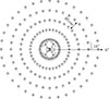 |
Figure 2. Drone setup in the hemi-anechoic room. |
At least one loudspeaker, termed “secondary source”, is required to synthesize a compensation signal to interfere destructively and thus reduce the drone noise. Since the aim of the ANC system is an SPL reduction in a target area, the sound reproduction requires a certain degree of spatial selectivity. Five Fostex 6301B active studio monitors were placed directly below the drone in a cross-like shape for this reason. The central loudspeaker in the middle pointed downwards, while the other four loudspeakers were placed on the four sides of the central loudspeaker tilted upwards at an angle of about 30°. The array is depicted in Figure 2b. It is important to note that the drone is no longer airworthy due to size and weight of this array. However, the focus of this study is on electro-acoustic properties rather than the flight performance.
The estimate of the far drone noise is based on a linear array with six DPA 4061 microphones and a constant spacing of 20 cm. These microphones are referred to as “error microphones”, because, with the ANC in place, they capture the remaining noise that constitutes the error of the cancellation. Because drones are usually located above the listener during operation, the microphone array was placed on the ground below the drone. An HRT I turntable from HEAD acoustics GmbH was used to rotate the array in increments of 10°, which allowed to measure the noise in a disk below the drone. Figure 3 visualizes all considered error microphone positions. The figure indicates that the absolute distance between microphones increases towards the outside of the disk. Although a total of 5 ⋅ 36 + 1 = 181 positions are considered, an ANC system might aim for an SPL reduction for only a subset of these positions if a specific listener position is available, effectively narrowing down the target area. The error microphones are used for ANC system design, but will not be available in the application for practical reasons. The vertical distance between the drone and error microphone array depends on the specific measurement setup, which is described in more detail in Section 3.
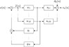 |
Figure 3. Top-down view of error microphone positions for the considered turntable angles. |
2.2 Digital system model
Sound pressure fields generated by moving surfaces are governed by non-linear differential equations, however, non-linear components are often excluded from analyses due to minor influence further away from the surface [9]. Interaction between the rotor blades can lead to slow time variations in the flow below the drone at rates of 10 Hz [44]. Here, we assume that non-linearities and time variations have negligible effect on signals captured by the reference microphones. Accordingly, this work is based on a digital-domain LTI system model. For this reason, any signal defined here denotes a digital quantity instead of a sound pressure wave. Analogously, magnitude spectra given in this work always relate to the digital signal. They are linked directly to pressure values with a corresponding calibration factor.
Throughout this paper a system may be referred to by its impulse response, Z-transform or discrete Fourier transform (DFT). Impulse responses are indicated by lower case letters, e.g. the primary path impulse response p. The corresponding Z-transform and DFT are denoted using uppercase letters with parenthesized z and f, respectively.
Figure 4 illustrates the model at hand, which does not explicitly include the primary paths  . More specifically, the secondary and feedback paths are modeled as LTI systems due to their inherent causality and the guaranteed broadband excitation. Neither of these aspects can be ensured for the primary path, which suggests the use of the raw disturbance signal to retain potentially non-linear aero-acoustic effects.
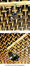 |
Figure 4. System-theoretic block diagram of feed-forward active noise control (ANC) system using the measured reference signal |

Other influences on the sound propagation that vary with time include wind and the motion of the drone. However, it is assumed that those influences affect the primary and secondary paths in the same way, while leaving the feedback mostly unaffected. The signal which would be captured by a reference microphone in the absence of secondary sources is denoted by x(n). This distinction is required to model the loudspeaker feedback on the measured reference signal  , which corresponds to x(n) with additive feedback from each loudspeaker during ANC system operation.
The error microphone signal at the remote location with index k is given by e
k
(n). The design target of the ANC system is to reduce the signal energy of the remaining noise, given by the sum of squared samples of e
k
(n) within the target region. The error signal e
k
(n) is composed of the corresponding primary disturbance signal d
k
(n), and a contribution of the feedforward system. The system consists of a multi-channel convolution of the measured reference signal  with all combinations of the feedforward filters w
m
and secondary paths s
k
m
for
with all combinations of the feedforward filters w
m
and secondary paths s
k
m
for  and
and  , respectively. M denotes the number of loudspeakers and K the number of error microphones. Here, s
k
m
denotes the secondary path impulse response that models sound propagation from loudspeaker m to the k-th error microphone. The impulse response of the feedforward filter that takes the measured reference signal as input and contributes to the signal of loudspeaker m is denoted by w
m
. Accordingly, e
k
(n) is given by
, respectively. M denotes the number of loudspeakers and K the number of error microphones. Here, s
k
m
denotes the secondary path impulse response that models sound propagation from loudspeaker m to the k-th error microphone. The impulse response of the feedforward filter that takes the measured reference signal as input and contributes to the signal of loudspeaker m is denoted by w
m
. Accordingly, e
k
(n) is given by
 (1)
(1)
The measured reference is afflicted by M loudspeaker-induced feedback signal components that lead to a recursive dependency. It is assumed that the feedback path is known exactly and can therefore be eliminated by an internal feedback within the feedforward ANC-system as described, e.g., in [29, 45, 46]. With this additional digital feedback, the measured reference signal  equals x(n). Stability considerations of this approach are analyzed in more detail in Section 5.4.
3 Measurements
The study aims to give insight into the acoustical behavior of drones in overhead hovering conditions with an application for drone ANC through acoustic measurements. These methods require information about the primary noise which drones emit, and the electro-acoustic transfer paths  and
and  . This information depends on the operating conditions and the positions of sensors, secondary sources and error microphones.
3.1 Measurement setup
Here, the setup described in Section 2.1 serves as an example of a drone-ANC system. Please note that for technical reasons, there was no loudspeaker array present during the Sentintel measurements. All measurements were carried out in the hemi-anechoic chamber of the Institute of Hearing Technology and Acoustics (IHTA) at RWTH Aachen University. Its dimensions are 11 m × 5.97 m × 4.5 m, and it is equipped with sound-proofing absorbers on all four walls and ceiling, except for a sound-reflecting floor. The drone was fixed to a contraption right below the sound-proofing absorbers on the ceiling. Cables for powering and controlling the drone and for connecting the sensors were set up along the ceiling, towards the nearest wall and down to a laptop computer on the ground. Instead of the drone’s internal flight control, an external brushless direct current (BLDC) control unit was used. The laptop controlled this unit by setting individual pulse-width modulation (PWM) values for each rotor. The same PWM value was applied to all rotors for simplicity. Slight variations between rotors result in similar but not identical BPFs. In addition, the BPF of a single rotor fluctuates over time, even if the PWM value remains constant.
An RME 12Mic microphone amplifier was used to record the signals of the sensors and error microphones simultaneously, using one internal clock running at a sampling frequency of 48 kHz. Note that phase synchronicity is important for phase-sensitive applications such as ANC. The data was transmitted to the laptop using the RME MADIface USB interface. This configuration enables an automatic iteration through different PWM values and rotational angles of the turntable.
Figure 2 illustrates the drone-related part of the measurement setup: Figure 2a depicts the arrangement for the primary noise measurements using the Sentinel. This setup was used to measure the primary noise of the DJI mini as well. Figure 2b shows the added loudspeaker array which enabled the measurement of the secondary and feedback paths. The measurement computer and microphone arrays are located below the drone, which is not visible in these images. A schematic view of the setup including the reference sensors and the secondary sources is given in Figure 5.
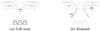 |
Figure 5. Schematic view showing the positions of reference sensors and secondary sources for the DJI mini and the Sentinel. |
3.2 Drone noise measurements
Starting the drone without the internal controller turned out to be challenging, especially with the folded rotors of the DJI mini, since the BLDC motor stops rotating when it gets out of synchronization. To combat this issue, we always started with the highest rotor speed. The DJI mini was recorded for 15 different rotor speeds, corresponding to BPFs between 179 Hz and 260 Hz for all rotational angles of the turntable. The Sentinel was recorded at 32 different rotor speeds, with BPFs ranging from 55 Hz to 124 Hz. In all cases, a short settling time was included to ensure that the drones reach a steady-state operation. The drone noise was subsequently captured for a duration of 2 s. The measurement software was configured to automatically wait for the turntable to complete the 10° turns. During this time, parts of the measured data could be saved to the laptop.
Figure 6 shows the smoothed magnitude spectrum of one example of the raw measurement data for three BPFs: 193 Hz, 223 Hz, and 247 Hz. More specifically, Figures 6a and 6b refer to the drone-mounted reference microphone and the innermost error microphone in the array, respectively. A moving average filter with ten samples was applied to the spectra for display purposes only. Due to sudden gusts of wind in the recorded data, they appear very noisy without filtering. Recall that the primary path  models the relationship between both of these figures.
 |
Figure 6. Smoothed magnitude spectrum of primary path-related measurement data for the DJI mini. |
The figures depict the typical tonal character of drone noise with spectral peaks at multiples of the BPF. However, it also reveals significant wind noise in the measured error signals at low frequencies. Its severity appears to increase with higher BPFs. Although the fundamental rotational frequencies are hardly visible due to the low-frequency wind noise, the BPFs are clearly visible in both, the reference and error signals. Note that e(n)=d(n) holds in this case because the measurement is conducted with an inactive ANC system.
Overall, the collected data for the DJI mini consist of sequences of 2 s length for 15 BPFs at 5 ⋅ 36 + 1 positions, and for the Sentinel to 2 s length for 32 BPFs at 5 ⋅ 36 + 1 positions. The different numbers of available BPFs is due to the rotors of the DJI mini losing synchronization of the BLDC controller. The corresponding reference signals are also included, one for the DJI Mini and two for the Sentinel.
3.3 Loudspeaker measurements
As shown in Figure 2b, the loudspeaker array was mounted below the DJI mini, for which the secondary paths  and feedback paths
  were identified from the measurement data. They are similar to well-known room impulse responses, but need to contain the effect of the loudspeaker for ANC purposes.
The five loudspeakers were measured individually using a logarithmic chirp signal [47] with a frequency range of 50 Hz to 20 kHz and a duration of 10 s. The loudspeakers’ amplification was fairly high, leading to an average total harmonic distortion of 4.84%, as was calculated using the method described in [48]. The loudspeaker signal was replayed over the headphone output of the microphone amplifier and simultaneously looped back digitally on a recording channel as a reference signal. This way, the digital delay of the measurement setup is not taken into account for simulation purposes. The effect of processing delay will be analyzed in Section 5.2. Again, each loudspeaker was recorded for each rotational angle of the turntable. This yields secondary path impulse responses for a total of 5 ⋅ 36 + 1 locations and 5 loudspeakers. Likewise, 1 ⋅ 5 and 2 ⋅ 5 feedback path impulse responses are available for the DJI mini and Sentinel, respectively.
We assume that the drone itself has only minor influence on the secondary paths  , which is why the same paths were used for the Sentinel and the DJI mini. This assumption is based on the fact that the mounts for the drone and loudspeaker array provide a significantly larger surface area than the drones themselves. The wind which the drones produce influence the sound propagation by increasing the propagation speed in the downwards direction. This effect could be investigated in future works using a flight-ready prototype.
3.4 Post processing
In this section, the identified secondary paths  and feedback paths
  are analyzed. In our previous work [43], we demonstrated the limited performance for primary-path estimation, which can be explained by tonal excitation and the presence of wind noise in the error-microphone signal. To avoid loss of information through an explicit system identification step, the primary path
  is considered implicitly by using the recordings of the disturbance directly.
Using the loudspeaker measurement data, finite impulse response (FIR) models of the electro-acoustic paths were identified from each loudspeaker to each reference microphone, and each error microphone position shown in Figure 3. The beneficial properties of the chirp excitation signal [47] were used to identify the impulse responses of  and
and  as FIR filters using spectrum division.
Figure 7 shows the impulse response of an exemplary secondary path corresponding to the path between the central loudspeaker and the inner-most microphone at a turntable angle of 0°. The figure illustrates a dead time of about 10 ms, which corresponds to a distance of 3.4 m at a speed of sound of 340 m/s. This value aligns with the room dimensions and the position of the drone relative to the error microphone array. The figure further shows the impulse response of the corresponding feedback path. Here, the dead time is smaller since the reference microphone is located close to the loudspeaker. Additionally, echos from the reflective floor are visible in the impulse response. Their time delay is again matching the vertical distance. Also, the amplitude of the feedback path is lower than the secondary path, indicating a negligible effect of feedback in the system considered. Note that the FIR filters identified are specific to the loudspeakers used and to the precise setup.
 |
Figure 7. Impulse responses of identified transfer paths. |
Figure 8 shows a comparison of all secondary paths from the center loudspeaker to the error-microphone array at a fixed turntable angle of 0°. Here, the difference in time delay increases going away from the center, as it is expected from the measurement setup. This further solidifies the plausibility of the estimated paths.
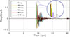 |
Figure 8. Comparison of estimated secondary paths at different distances to the center of the turntable. |
4 Filter optimization
As introduced in Section 2.2, an LTI system model is used for the design and analysis of a drone-mounted feedforward ANC system. For technical reasons, the drone was already running when the microphone recordings started. Therefore, padding the reference signal with zeroes at the beginning gives sub-optimal results. For this reason, only those samples of the convolution sequence (cf. Eq. (1)) are considered, for which sufficiently many previous samples of the reference signal are known. The minimum mean-squared error (MMSE) optimization of the feedforward filters otherwise follows the approach outlined in [49]. Throughout this section, different objective functions are used for targeted ANC and global ANC, where “global” refers to all positions given by Figure 3. The goal of the targeted system is to reduce the remaining error at a specific position. The objective function to be minimized in this case is given by
 (2)
(2)
The sum of all targeted objectives serves as the objective function for the global system. It is given by
 (3)
(3)
Due to the spacing of the error microphones (see Fig. 3), the center of the disk underneath the drone is favored using the objective function in equation (3). This focus could be shifted using additional weights for the individual target loss terms, which exceeds the scope of this paper. The optimization variables correspond, in all cases, to the unknown filter coefficients w m n of the FIR filter. The unique set of optimal coefficients w m for all indices m and time instants n are obtained by setting
 (4)
(4)
where ℒ* stands for either of the targeted or the global objective functions. The samples of the error-microphone signals e k (n) depend linearly on the unknown filter coefficients w m n . For this reason equation (4) is also linear in the filter coefficients. This problem can be solved using well-researched numerical tools [50]. Concretely, the filter coefficients can be retrieved from a matrix-vector product. In this case, the pseudoinverse of a block-matrix made up of convolution matrices and a vector of appropriately stacked error signals. Each convolution matrix is constructed from a reference signal filtered using a secondary path yielding one matrix for each combination.
Concretely, the remaining error at the specific position k from equation (1) can be rewritten in vector form as
 (5)
(5)
Here, the curly braces indicate a convolution matrix constructed from the embraced signal. A concrete example is
 (6)
(6)
All error vectors can be stacked to produce a single system of linear equations:
 (7)
(7)
The combined matrix H has a convenient structure that admits a fast solution even for large systems where all virtual microphone positions are considered. The general solution to equation (4) is given by
 (8)
(8)
Here, the star index represents the index k for a targeted solution using the system described in equation (9) or nothing in the case of a global solution using equation (7d).
We did not encounter numerical issues during the design of the filters. Depending on the resulting matrix, additional regularization can be helpful for improving the condition number.
4.1 Performance metric
In the following, the active attenuation
 is used as a performance metric. That is, the ratio of the energy spectra of the disturbance signal
  and the error signal
  , i.e.
 (9)
(9)
for the targeted system, and
 (10)
(10)
for the global system. Here,  and
and  denote the DFT of the disturbance signal d
k
and the error-signal e
k
at a specific error-microphone position, denoted by k, respectively. Since the magnitude spectra of the raw-data are noisy (cf. Fig. 6) they were additionally smoothed by applying 20th octave filters.
denote the DFT of the disturbance signal d
k
and the error-signal e
k
at a specific error-microphone position, denoted by k, respectively. Since the magnitude spectra of the raw-data are noisy (cf. Fig. 6) they were additionally smoothed by applying 20th octave filters.
5 Case study
The size, speeds and spacing of the two drone’s rotors are so different that a direct comparison of the results is not meaningful. Two drones were used instead of one to give an additional example. The results presented in this section are not intended to show a preference for one drone over the other.
The comprehensive measurement data allows to study the efficacy of feedforward ANC systems in the considered setup, which considers a drone ANC system that lacks error microphone data during operation. The use of fixed filters is justified by the fact that only the drones’ own noise is to be controlled. Here, the relative positions of the primary source, the reference sensors, and the secondary sources never change. We used recordings of the reference and error microphones, together with secondary paths estimated from separate recordings with a loudspeaker array, to design FIR filters for the active reduction of SPL at different target locations. Here, it is assumed that the secondary paths remain constant with respect to time and drone operation, i.e. are not affected by the resulting airflow. For the purposes of this case study, only a single BPF is considered for each drone. Here, 97 Hz and 223 Hz were chosen for the Sentinel and the DJI mini, respectively. As shown in Figure 5, the ANC system of the Sentinel uses two reference sensors whereas the one of the DJI uses only one.
5.1 Effect of filter length
One important parameter is the length of the fixed filters N w , which this section investigates for both drones by evaluating the maximum active attenuation achieved by the globally optimized ANC system over all DFT-frequencies f. In all cases, the filters were designed using the MMSE criterion presented in the previous section. However, to avoid overfitting to the recorded data, the design and evaluation were carried out on separate halves of the drone noise recordings. The goal of this methodology is to asses the feasibility of deploying a “blind” system with no access to the error microphones. However, the second half of the same measured sequence may not be a faithful representation of all possible data encountered during deployment.
Nonetheless, the system can be designed and evaluated as described using the measurement data, giving the results shown in Figure 9a. The attenuation is averaged in space over all virtual microphone positions and the spectral peak is considered (i.e., the maximum of  ). Although the peak attenuation generally increases with the filter length up to 2048 samples, the increase is not monotonous because ℒ considers the wide-band signal. Due to the observed stagnation, a filter length Nw = 2048 is used for the remainder of the paper. At a sampling rate of 48 kHz, a filter length Nw = 2048 corresponds to about 42.67 ms.
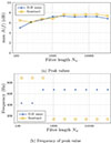 |
Figure 9. Spectral peak of spatially averaged active attenuation over varying length Nw of the control filters. |
Figure 10 shows the squared magnitude spectra of the spatially averaged disturbance and residual error signals for a filter length of Nw = 2048. Additionally, the performance of an unconstrained system is shown. This non-physical system does not require reference signals but uses knowledge about future data to replay signals over the loudspeakers that optimally attenuate the disturbance. It should therefore be interpreted as an upper performance bound that is independent of the choice of reference sensors. The figure shows that the attenuation is focused around the spectral peaks that are above the wind noise and below a few kilohertz. The unconstrained model reveals that the wind-noise cannot be attenuated by the system even without the causality constraint. Alternatively, this reveals low correlation between the wind noise contributions at different error microphones. The peak in signal power at about 15.6 kHz can be attributed to the electric motor control and cannot be attenuated globally using this method. Also, note that the curves in Figure 10 are smooth compared to Figure 6, which is due to the spatial averaging and the 20th octave band filtering.
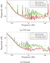 |
Figure 10. Spatially averaged squared magnitudes of disturbance signals d(n) and error signals e(n) in 20th octave bands. |
The acoustic loudness was determined for the drone noise with and without the ANC system using the method described in [51]. The perceived loudness was reduced by 8.5% and 6.5% on average for the DJI and the Sentinel, respectively. For this evaluation, all virtual microphone positions were considered independently as diffuse sources. Please note, that these results were calculated from the digital levels by using a calibration factor derived from the sensitivities and gains given by the manufacturers of the devices used and may therefore be slightly inaccurate.
5.2 Effect of processing delay
The position of the reference sensors is between the rotor and the secondary sources. This way the primary noise always reaches the reference sensor before the secondary sources. This advantage can be significantly reduced due to large processing delays. We simulated additional delay by shifting the secondary paths. Due to the assumed system model it does not make a difference whether the delay is applied before or after application of the control filters.
The results in Figure 11 demonstrate the resilience of the chosen metric against additional delay. The choice of filter length has a much higher influence on the performance. This is likely due to the rather tonal excitation which can be predicted well using linear filters.
 |
Figure 11. Spectral peak of spatially averaged active attenuation over additional processing delay. |
5.3 Effect of target location
The targeted ANC system is evaluated for all error microphones shown in Figure 3. The same methodology of splitting the measured sequences from Section 5.1 was used here. This evaluation reveals the distribution of uncorrelated noise at the error microphones and can be used as a reference for adjusting weighting coefficients in subsequent work.
Figure 12 shows the maximum of the attenuation  for all error-microphone positions for both drones. For the DJI mini, the resulting pattern indicates jumps in performance at neighboring angles. This can be explained by the fact that different angles correspond to different measurements with slightly different conditions due to fluctuations in the wind noise. The results for the Sentinel, however, show a pattern in the radial direction. A darker ring, corresponding to lower peak attenuation, can be observed at a radius corresponding to 40 cm. One explanation for this is the increased amount of wind right below the rotors that interfere with the BPF peak. The large loudspeaker array would probably have blocked a significant amount of the wind. However, it was not present during the recordings. Additionally the presence of the loudspeaker array would lead to wind noise production close to the reference sensors which could explain the higher maximum active attenuation for the Sentinel.
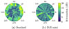 |
Figure 12. Peak active attenuation in 20th octave band at varying target location. |
To gain further insight into the spatial variability of the attenuation, Figure 13 jointly visualizes the attenuation values from Figure 12 as a histogram. The figure suggests that the median peak attenuation within the disk with one meter radius and a vertical distance of about 3.4 m is close to 9.4 dB. The maximum achievable attenuation is biased due to the wind noise, which is visible in Figure 10b. Here, the peak at the BPF cannot be reduced below the noise floor given by the wind noise ramp. For this reason, the attenuation of actual sound may be greater than the values given here.
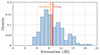 |
Figure 13. Histogram of peak attenuation values from simulations using only one error microphone. |
5.4 Influence of the feedback path
Since the distance between drone-mounted loudspeakers and microphones is necessarily small, acoustic feedback must be anticipated. This is modeled by the feedback path q according to Figure 4, which can lead to a performance degradation or instability if not accounted for. Both of these aspects are addressed here. The previous experiments assumed that its influence is compensated. By dropping this assumption, we investigate its influence for the present application.
Figure 4 shows that all loudspeakers, each corresponding to one of the M channels, contribute a feedback term to the measured reference signal  . The signals x(n) and
  are therefore related recursively according to
 (11)
(11)
Clearly,  approaches x(n) when the convolution of the filters w
m
and the feedback paths q
m
has a low amplitude. To investigate if this holds in the present application, the same filters that produce the results which Figure 10a depicts are considered as an example. Figure 14a shows the magnitude response contribution which is jointly caused by all feedback paths. The so-called feedback loop gain for this system is given by
approaches x(n) when the convolution of the filters w
m
and the feedback paths q
m
has a low amplitude. To investigate if this holds in the present application, the same filters that produce the results which Figure 10a depicts are considered as an example. Figure 14a shows the magnitude response contribution which is jointly caused by all feedback paths. The so-called feedback loop gain for this system is given by
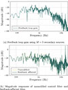 |
Figure 14. Influence of the loudspeaker feedback on feedforward control. A control filter is compared with the corresponding combined filter with additional digital feedback cancellation as an example. |
 (12)
(12)
The figure reveals a low feedback loop gain for a large part of the frequency spectrum, with peaks of less than −10 dB at about 480 Hz, 700 Hz and 2000 Hz.
Based on the measured feedback paths, the effect on the overall system can be evaluated by integrating the feedback-afflicted measurement signal  into the feedforward filter transfer function. This yields “feedback-afflicted” feedforward filters
 (13)
(13)
for all channels  . These filters take the effect of feedback into account.
Figure 14b shows the magnitude responses of the designed filter  and the feedback-afflicted filter
  . The figure reveals that both filters are almost identical. The observed peak magnitude deviation amounts to less than 2.5 dB, and is almost zero for a large part of the spectrum. Moreover,
  is stable because the magnitude of the internal feedback loop gain, shown in Figure 14a, is less than 0 dB at all frequencies [52]. Here, the change in filter coefficients is so small that the change in performance resulting from the use of the feedback afflicted filters is insignificant.
In summary, the influence of the feedback path turned out to be minor in our experiments. It could be neglected due to its low impact on the results. This surprisingly low impact can be explained by the downward orientation and the directivity of the loudspeakers used. The fact that loudspeakers and microphones can be arranged in such a way is an advantage of drone-mounted ANC systems. In contrast to other systems such as [29], which inherently require feedback compensation, the loudspeaker-microphone combination in drone-mounted ANC systems can be chosen to mitigate the feedback problem. However, the loudspeakers are not mounted to the frame directly (see Fig. 2b) which leads to low mechanical coupling. For this reason, the amount of feedback may be higher in practice.
6 Conclusion
This contribution demonstrates initial results in the field of spatial ANC for drones, where the reference microphones and secondary sources are mounted on the drone. It involved the construction of drone-ANC prototypes, on which extensive measurements were conducted regarding primary and secondary sound propagation. The results of the measurements are used to implement a simulation framework based on fixed FIR filters. The filter coefficients are determined by minimizing the sum of squared samples of the residual error signals using a reference recording. To validate the feasibility of fixed filters, different recordings are used for the filter design and the evaluation. This demonstrates a spatially robust median active attenuation of tonal drone noise components of 9.4 dB with peak attenuation values above 15 dB. These results suggest the principal feasibility of such a system. The study suggests that ANC can be an attractive method for reducing the noise pollution of drones, for example in urban use cases. Future research should focus on fine-tuning the hardware regarding its amount, capability and robustness during flight. The methodology presented in this paper can be applied to other prototypes with different hardware configurations for evaluating ANC capabilities.
Acknowledgments
We would like to thank the ITHA team – Prof. Dr.-Ing. Janina Fels, Dr.-Ing. Lukas Aspöck, Marc Eiker and Thomas Schaefer for their assistance with our measurements and for granting access to the hemi-anechoic chamber.
Funding
This work was part of the SILENce project which was funded by mFund of the German Federal Ministy of Digital and Transport (BMDV).
Conflicts of interest
The authors declare no conflict of interest.
Data availability statement
The research data associated with this article are available in Zenodo, under the reference https://doi.org/10.5281/zenodo.16965878.
References
- J. Scott, C. Scott: Drone delivery models for healthcare, in: Proceedings of the Hawaii International Conference on System Sciences (HICSS) Held in Hawaii, USA, 2017, pp. 3297–3304. [Google Scholar]
- G. Attenni, V. Arrigoni, N. Bartolini, G. Maselli: Drone-based delivery systems: a survey on route planning. IEEE Access 11 (2023) 123476–123504. [Google Scholar]
- F. Betti Sorbelli: UAV-based delivery systems: a systematic review, current trends, and research challenges. Journal on Autonomous Transportation Systems 1 (2024) 1–40. [Google Scholar]
- V.C. Hollman: Drone photography and the re-aestheticisation of nature, in: Decolonising and Internationalising Geography: Essays in the History of Contested Science, 2020, pp. 57–66. [Google Scholar]
- S. Zhao: The role of drone photography in city mapping, in: Proceedings of the International Conference on Application of Intelligent Systems in Multi-modal Information Analytics Held in Changzhou, China, 2020, pp. 343-348. [Google Scholar]
- V. Puri, A. Nayyar, L. Raja: Agriculture drones: a modern breakthrough in precision agriculture. Journal of Statistics and Management Systems 20 (2017) 507–518. [CrossRef] [Google Scholar]
- Mehrzad, A.D. Reza, Y. Seung-Hwa, C. Yong, L. Jeekeun: Characteristics of a tip-vortex generated by a single rotor used in agricultural spraying drone. Experimental Thermal and Fluid Science 149 (2023) 110995. [Google Scholar]
- S. More, P. Davies: Human responses to the tonalness of aircraft noise. Noise Control Engineering Journal 58 (2010) 420. [Google Scholar]
- F. Farassat: Derivation of Formulations 1 and 1A of Farassat. NASA Langley Research Center, 2007. [Google Scholar]
- L. Gutin: On the sound field of a rotating propeller. Physical Magazine of the Soviet Union 9 (1948). [Google Scholar]
- R. Cabell, F. Grosveld, R. McSwain: Measured noise from small unmanned aerial vehicles, in: Proceedings of the Inter-Noise and Noise-Con Congress and Conference Held in Providence, Rhode Island, 2016, pp. 345-354. [Google Scholar]
- Dreier, M. Vorländer: Drone auralization model with statistical synthesis of amplitude and frequency modulations. Acta Acustica 8 (2024) 35. [Google Scholar]
- A.J. Torija, P. Chaitanya, Z. Li: Psychoacoustic analysis of contra-rotating propeller noise for unmanned aerial vehicles. The Journal of the Acoustical Society of America 149 (2021) 835–846. [CrossRef] [PubMed] [Google Scholar]
- R. König, L. Babetto, A. Gerlach, J. Fels, E. Stumpf: Prediction of perceived annoyance caused by an electric drone noise through its technical, operational, and psychoacoustic parameters. The Journal of the Acoustical Society of America 156 (2024) 1929–1941. [Google Scholar]
- M. Lotinga, M. Green, A.J. Torija Martinez: How do flight operations and ambient acoustic environments influence noticeability and noise annoyance associated with unmanned aircraft systems? in: Proceedings of Quietdrones Held in Manchester, UK, 2024. [Google Scholar]
- Schäffer, R. Pieren, K. Heutschi, J.M. Wunderli, S. Becker: Drone noise emission characteristics and noise effects on humans-A systematic review. International Journal of Environmental Research and Public Health 18 (2021) 5940. [CrossRef] [PubMed] [Google Scholar]
- Rascon, J. Martinez-Carranza: A review of noise production and mitigation in UAVs. Machine Learning for Complex and Unmanned Systems (2024) 220–235. [Google Scholar]
- F.B. Metzger: An assessment of propeller aircraft noise reduction technology. NASA Langley Research Center, 1995. [Google Scholar]
- Cambray, E. Pang, S.A.S. Ali, D. Rezgui, M. Azarpeyvand: Investigation towards a better understanding of noise generation from UAV propellers, in: Proceedings of the AIAA/CEAS Aeroacoustics Conference Held in Atlanta, Georgia, 2018, p. 3450. [Google Scholar]
- J. Du Plessis, A. Bouferrouk: Aerodynamic and aeroacoustic analysis of looped propeller blades, in: Proceedins of AIAA/CEAS Aeroacoustics Conference Held in Rome, Italy, 2024. [Google Scholar]
- X. Kong, M. Kingan, H. Zhu: The effect of strut geometry on propeller-strut interaction tone noise, in: Proceedings of Quietdrones Held in Manchester, UK, 2024. [Google Scholar]
- Miljković: Methods for attenuation of unmanned aerial vehicle noise, in: Proceedings of the International Convention on Information and Communication Technology, Electronics and Microelectronics (MIPRO) Held in Opatija, Croatia, 2018, pp. 914-919. [Google Scholar]
- M.V. Mane, P.D. Sonawwanay, M. Solanki, V. Patel: A comprehensive review on advancements in noise reduction for unmanned aerial vehicles (UAVs). Journal of Vibration Engineering & Technologies 12 (2024) 1375–1397. [Google Scholar]
- M. Larsson: Active Noise Control in Ventilation Systems: Practical Implementation Aspects. Blekinge Institute of Technology, 2008. [Google Scholar]
- H.F. Olson, E.G. May: Electronic sound absorber. The Journal of the Acoustical Society of America 25 (1953) 1130–1136. [CrossRef] [Google Scholar]
- M. Bai, D. Lee: Implementation of an active headset by using the H ∞ robust control theory. The Journal of the Acoustical Society of America 102 (1997) 2184–2190. [Google Scholar]
- J. Zhang, T.D. Abhayapala, W. Zhang, P.N. Samarasinghe, S. Jiang: Active noise control over space: a wave domain approach. IEEE/ACM Transactions on Audio, Speech, and Language Processing 26 (2018) 774–786. [Google Scholar]
- B. Rafaely: Fundamentals of Spherical Array Processing. Springer, 2015. [Google Scholar]
- M. Budnik, V. Mees: Free field active noise control system development using a 3D finite element based approach. Acta Acustica 9 (2025) 37. [Google Scholar]
- S. Koyama, J. Brunnström, H. Ito, N. Ueno, H. Saruwatari: Spatial active noise control based on kernel interpolation of sound field. IEEE/ACM Transactions on Audio, Speech, and Language Processing 29 (2021) 3052–3063. [Google Scholar]
- H. Sun, C.T. Jin, T.D. Abhayapala, P. Samarasinghe: Active noise control over 3D space with a dynamic noise source, in: Proceedings of the International Conference on Acoustics, Speech and Signal Processing (ICASSP) Held in Seoul, Korea, 2024, pp. 1236-1240. [Google Scholar]
- H. Bi, F. Ma, T.D. Abhayapala, P.N. Samarasinghe: Spherical sector harmonics based directional drone noise reduction, in: Proceedings of the International Workshop on Acoustic Signal Enhancement (IWAENC) Held in Bamberg, Germany, 2022, pp. 1-5. [Google Scholar]
- H. Bi, Y. Zhan, T.D. Abhayapala, P.N. Samarasinghe: Directional active noise control for drone noise reduction. JASA Express Letters 5 (2025) 124801. [Google Scholar]
- S.M. Kuo, D.R. Morgan: Active noise control: a tutorial review. Proceedings of the IEEE 87 (1999) 943–973. [Google Scholar]
- V. Valimaki, A. Franck, J. Ramo, H. Gamper, L. Savioja: Assisted listening using a headset: enhancing audio perception in real, augmented, and virtual environments. IEEE Signal Processing Magazine 32 (2015) 92–99. [Google Scholar]
- S.M. Kuo, H. Chuang, P.P. Mallela: Integrated automotive signal processing and audio system. IEEE Transactions on Consumer Electronics 39 (1993) 522–532. [Google Scholar]
- Hilgemann, E. Chatzimoustafa, P. Jax: Data-driven uncertainty modeling for robust feedback active noise control in headphones. Journal of the Audio Engineering Society (2024) 873–883. [Google Scholar]
- M.A. Poletti: Three-dimensional surround sound systems based on spherical harmonics. Journal of the Audio Engineering Society 53 (2005) 1004–1025. [Google Scholar]
- J. Ahrens, R. Rabenstein, S. Spors: The theory of wave field synthesis revisited, in: Proceedings of the Audio Engineering Society Convention Held in Amsterdam, The Netherlands, 2008. [Google Scholar]
- T. Kojima, K. Arikawa, S. Koyama, H. Saruwatari: Multichannel active noise control with exterior radiation suppression based on Riemannian optimization, in: Proceedings of the European Signal Processing Conference (EUSIPCO) Held in Helsinki, Finland, 2023, pp. 96-100. [Google Scholar]
- G.A. Brès, K.S. Brentner, G. Perez, H.E. Jones: Maneuvering rotorcraft noise prediction. Journal of Sound and Vibration 275 (2004) 719–738. [Google Scholar]
- W.N. Manamperi, T.D. Abhayapala, L. Birnie, J. Zhang, P.N. Samarasinghe: Drone audition: on measurements and modeling of drone-related transfer functions. IEEE Transactions on Audio, Speech and Language Processing (2025). [Google Scholar]
- J. Steiner, F. Hilgemann, P. Jax: Empirical study on active noise control in UAVs, in: Proceedings of the 11th Convention of the European Acoustics Association Forum Acusticum Held in Malaga, Spain, 2025. [Google Scholar]
- Y. Wu, D. Casalino: Numerical investigation of aeroacoustics for side-by-side rotor operating in proximity to the ground, in: Proceedings of Quietdrones Held in Manchester, UK, 2024. [Google Scholar]
- J. Hellgren, F. Urban: Bias of feedback cancellation algorithms in hearing aids based on direct closed loop identification. IEEE Transactions on Speech and Audio Processing 9 (2001) 906–913. [Google Scholar]
- C. Weyer, P. Jax: Feedback-aware design of an occlusion effect reduction system using an earbud-mounted vibration sensor, in: Proceedings of the 15th ITG Conference on Speech Communication Held in Aachen, Germany, 2023, pp. 225-229. [Google Scholar]
- S. Müller, P. Massarani: Transfer-function measurement with sweeps. Journal of the Audio Engineering Society 49 (2001) 443–471. [Google Scholar]
- Farina: Simultaneous measurement of impulse response and distortion with a swept-sine technique, in: Proceedings of the 108th AES Convention, Paris, France, 2000. [Google Scholar]
- O. Kirkeby, P.A. Nelson: Digital filter design for inversion problems in sound reproduction. Journal of the Audio Engineering Society 47 (1999) 583–595. [Google Scholar]
- G.H. Golub, C.F. Van Loan: Matrix Computations. Johns Hopkins University Press, 1996. [Google Scholar]
- ISO 532-2:2017(E): “Acoustics - Methods for calculating loudness - Part 2: Moore-Glasberg method”. International Organization for Standardization. [Google Scholar]
- Chottera, G. Jullien: A linear programming approach to recursive digital filter design with linear phase. IEEE Transactions on Circuits and Systems 29 (1982) 139–149. [Google Scholar]
Data from our previous work [43] is available under https://www.doi.org/10.5281/zenodo.15064305.
The revised database is available under https://zenodo.org/records/16965878.
Cite this article as: Steiner J. Hilgemann F. & Jax P. 2026. Investigations on drone-mounted active noise control. Acta Acustica, 10, 32. https://doi.org/10.1051/aacus/2026030.
All Figures
|
Figure 1. Schematic layout of a drone with additional hardware required for active noise control (ANC). Primary ( |
| In the text | |
|
Figure 2. Drone setup in the hemi-anechoic room. |
| In the text | |
|
Figure 3. Top-down view of error microphone positions for the considered turntable angles. |
| In the text | |
|
Figure 4. System-theoretic block diagram of feed-forward active noise control (ANC) system using the measured reference signal |
| In the text | |
|
Figure 5. Schematic view showing the positions of reference sensors and secondary sources for the DJI mini and the Sentinel. |
| In the text | |
|
Figure 6. Smoothed magnitude spectrum of primary path-related measurement data for the DJI mini. |
| In the text | |
|
Figure 7. Impulse responses of identified transfer paths. |
| In the text | |
|
Figure 8. Comparison of estimated secondary paths at different distances to the center of the turntable. |
| In the text | |
|
Figure 9. Spectral peak of spatially averaged active attenuation over varying length Nw of the control filters. |
| In the text | |
|
Figure 10. Spatially averaged squared magnitudes of disturbance signals d(n) and error signals e(n) in 20th octave bands. |
| In the text | |
|
Figure 11. Spectral peak of spatially averaged active attenuation over additional processing delay. |
| In the text | |
|
Figure 12. Peak active attenuation in 20th octave band at varying target location. |
| In the text | |
|
Figure 13. Histogram of peak attenuation values from simulations using only one error microphone. |
| In the text | |
|
Figure 14. Influence of the loudspeaker feedback on feedforward control. A control filter is compared with the corresponding combined filter with additional digital feedback cancellation as an example. |
| In the text | |
Current usage metrics show cumulative count of Article Views (full-text article views including HTML views, PDF and ePub downloads, according to the available data) and Abstracts Views on Vision4Press platform.
Data correspond to usage on the plateform after 2015. The current usage metrics is available 48-96 hours after online publication and is updated daily on week days.
Initial download of the metrics may take a while.