| Issue |
Acta Acust.
Volume 9, 2025
|
|
|---|---|---|
| Article Number | 72 | |
| Number of page(s) | 10 | |
| Section | Computational and Numerical Acoustics | |
| DOI | https://doi.org/10.1051/aacus/2025057 | |
| Published online | 25 November 2025 | |
Technical & Applied Article
Transmission line matrix model: numerical dispersion effects on simulated specular reflection
1
UMRAE, CEREMA, Univ Gustave Eiffel, F-67035 Strasbourg, France
2
UMRAE, Univ Gustave Eiffel, CEREMA, F-44344 Bouguenais, France
* Corresponding author: This email address is being protected from spambots. You need JavaScript enabled to view it.
Received:
7
February
2024
Accepted:
17
October
2025
Abstract
Numerical sound propagation models include a wide range of methods with their own advantages depending on the physical phenomena under consideration. Due to its low-order scheme characteristic, the transmission line matrix (TLM) model is considered for coarse modeling of sound fields in complex outdoor environments. However, the space-time integration scheme of the method is dispersive and affects the free-field predictions. This paper extends a previous study of the numerical dispersion effect on the acoustic pressure field. An ideal case with specular reflections on a perfectly reflective ground is considered to represent the worst-case scenario, as the absence of absorption by the boundary maximizes the influence of numerical dispersion. First, a reminder of the model boundary conditions for specular reflection is provided, and the corresponding analytical solution is introduced as a reference to evaluate the reliability of the model. Then, a numerical experiment is presented and performed for different sound source characteristics. The result analysis shows that dispersion can induce misplaced interferences in the numerically simulated sound fields and the resulting errors are quantified in terms of sound pressure levels (SPL). Finally, an analytical comparison with a well-known finite difference numerical scheme gives a perspective on the TLM model performance regarding several applications.
Key words: Transmission line matrix method / Numerical methods / Outdoor sound propagation / Numerical dispersion / Interference / Reflections
© The Author(s), Published by EDP Sciences, 2025
 This is an Open Access article distributed under the terms of the Creative Commons Attribution License (https://creativecommons.org/licenses/by/4.0), which permits unrestricted use, distribution, and reproduction in any medium, provided the original work is properly cited.
1 Introduction
Although the negative impact of noise pollution on human health is established [1], the effects of anthropogenic noise on biodiversity are under study [2, 3]. Researching the impact of noise on wildlife communications (mainly birds and mammals) brings together various scientific fields and leads to cooperations. The study of sound propagation in forests is part of this effort because it can support in-situ recordings of sound signals made by eco acousticians [4]. To better address this topic, several long-range outdoor sound propagation models are available and provide quantitative noise predictions. Usually, noise maps are produced using physics-based engineering methods which present limitations in specific cases, e.g. for porous ground and/or diffuse field [5].
More generally, outdoor sound environment modeling is frequently performed with a large panel of numerical methods, presenting various advantages and limitations, either wave-based methods in the time domain (e.g. FDTD) or wave-based methods in the frequency domain (e.g. BEM, PE) or analytical methods (e.g. Weyl–Van der Pol formulation) or ray-tracing methods [6–8]. Depending on the specificities (symmetry, frequency range...) of the scenario to be modeled, frequency domain, time domain or modal decomposition methods can be chosen for their assets [8, 9]. Among these methods, the Boundary Element Method (BEM) stands out for its efficiency in boundary-dominated scenarios, as it avoids numerical dispersion errors within the volume and requires discretization of only the boundaries, reducing the dimensionality of the problems by one. However, the Transmission Line Matrix (TLM) method is considered to model complex sound environments with a high number of reflections (such as with tree trunks in forests) using impedance boundary conditions. Its computational cost scales with the size of the domain, but it is better suited to handle broadband scenarios with in-volume complexities. The low order characteristic of this scheme and its implementation makes it a potential candidate to solve the wave equation on such scenarios taking into account the backscattered components of the sound field [10, 11]. It has already been used to model realistic outdoor propagation with meteorological effects or multiple reflections by cylinder arrays normal to an impedance plane [12, 13] with source-receiver distances on the order of hundreds of times the minimum modeled wavelength [14].
The main issue of using a low-order spatial integration scheme, such as TLM or centered finite differences in the time domain (FDTD) on a Cartesian mesh is the apparition of numerical dispersion [15]. This pure discretization-induced artifact leads to spurious waves whose phase and group speeds depend on frequency [16]. To solve this problem, there are techniques to avoid or reduce numerical dispersion but all of them have a cost in either efficiency or complexity. For instance, increasing the number of points in a fixed-order FDTD scheme and optimizing the numerical dispersion equation is commonly done in aeroacoustics [17, 18]. For the TLM method, attempts have been made to modify the geometry of the mesh, but it increases the complexity of the implementation [19, 20]. In most cases, the method remains second-order, with the computational complexity similar to that of a matrix-vector product [11]. The effect of the numerical dispersion on TLM results has been highlighted from the free-field case [11]. This paper investigates the performance with respect to a singular reflection to assess the impact of numerical dispersion on the modeling of boundaries. This is a step toward realistic simulations of sound propagation in forests.
The study presented below focuses on the TLM model and its limitations in specific application domains. Instead of increasing the order of the model (i.e. numerical complexity at the boundaries), this paper thoroughly analyzes the effect of numerical dispersion on long-range modeling with specular reflection included. The approach aims to understand how much numerical dispersion affects the results so that the low-order scheme can be used knowingly.
First, a brief overview, complementary to the literature, is given on the theory and the implementation process of a boundary condition in the TLM method. Then the analytical solution of the specific case considered is given, together with some implementation details. Next, the setup of the numerical experiment is presented, and the results are analyzed for three different sound source characteristics. Finally, a theoretical comparison between the TLM model and a common FDTD method is given in the last part.
2 Theoretical background
The TLM method is based on the Huygens-Fresnel wavefront decomposition to model the propagation of sound waves within a fluid as an iterative process of spreading pressure pulses through a Cartesian mesh [21]. The simulated domain is decomposed into transmission lines connecting nodes located by the vector of indices:  where d is the dimension of the problem. The spatial step Δℓ between the lines is equal in every Cartesian directions and the time is decomposed into steps Δt such as
  . This nomenclature allows writing the incident pressure pulse to the node r along the line m ∈ {1,…,2d} at the time step n as
  . Similarly,
  represents the scattered pulse reflected instantaneously. From their modelling, it is possible to calculate
n
P
r
, an approximated value of the exact acoustic pressure p(x
1,…,x
d
,t
n
) taken at the point (x
1, …, x
d
) at time t
n
.
represents the scattered pulse reflected instantaneously. From their modelling, it is possible to calculate
n
P
r
, an approximated value of the exact acoustic pressure p(x
1,…,x
d
,t
n
) taken at the point (x
1, …, x
d
) at time t
n
.
2.1 Relation to the wave equation
Deriving from the TLM model pressure pulses definition, the equivalent numerical pressure scheme can be formulated as follows [11]:
![Mathematical equation: $$ \begin{aligned} _{n+1}P_\mathbf{r}+_{n-1}P_\mathbf{r} =&\frac{1}{d}\sum _{m=1}^d \Big [_{n}P_{\left(j_1+\delta _{m1}, \dots , j_d+\delta _{md} \right)} \nonumber \\&+ _{n}P_{\left(j_1-\delta _{m1}, \dots , j_d-\delta _{md} \right)}\Big ], \end{aligned} $$](/articles/aacus/full_html/2025/01/aacus240023/aacus240023-eq17.gif) (1)
(1)
where δ denotes the Kronecker delta. To analyze the order of approximation of this scheme, and to derive the solved wave equation, Taylor expansions are applied to all the terms of equation (1) [14, 21], leading to:
 (2)
(2)
where  . This reveals the wave equation and shows that the TLM model is a second-order approximation method in both time and space. It also highlights that the TLM solves the wave equation only if the condition c
2
TLM = c
0
2 is satisfied. Expanding this condition yields:
. This reveals the wave equation and shows that the TLM model is a second-order approximation method in both time and space. It also highlights that the TLM solves the wave equation only if the condition c
2
TLM = c
0
2 is satisfied. Expanding this condition yields:
 (3)
(3)
which corresponds with the Courant–Friedrichs–Lewy (CFL) stability condition of the so-called finite difference Leap-Frog scheme [7].
2.2 Numerical dispersion
To assess the model stability, the numerical dispersion relation of the method can be expressed as:
 (4)
(4)
This equation indicates that the TLM method is unconditionally stable in a homogeneous, non-dissipative medium. However, it also reveals that the model exhibits numerical dispersion along the primary grid directions (e.g., in the 2D case,  , where θ is the angle between the plane wave vector and the horizontal direction of the grid). Equation (4) is equivalent to the dispersion relation of a second-order FDTD scheme centered in space and time. More theoretical aspects of the homogeneous and inhomogeneous TLM model are thoroughly described for the free field case in [11]. The following will focus on the modeling of a reflection boundary condition within the method.
2.3 Reflection condition
To model a simple specular interaction on a reflective boundary, the TLM model uses a pressure reflection coefficient [22]. Compared to the free-field connection laws [11], the formula governing the transmission line between a boundary and the nearest node (Fig. 1) is modified as described in equation (5). Figure 1 shows additionally that the considered node is located at a distance Δℓ/2 from the boundary. This specificity ensures synchronization between the arrival of pulses reflected from a boundary and the regular pulses traveling along transmission lines of length Δℓ.
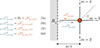 |
Figure 1. Representation of the 2D simple boundary reflection at the local node r = (j1, j2) close to a boundary of reflection coefficient R1. On the line m = 1, scattered pulse “S” (orange) at time step n becomes a reflected incident pulse “I” (blue) at next step n+1. |
The energetic absorption coefficient α for the boundary is described by:
 (6)
(6)
where Rm corresponds to the plane wave reflection coefficient assigned to the boundary perpendicular to the branch m. The condition Rm = 1 describes an infinitely rigid boundary (zero particle velocity), Rm = −1 a free boundary (zero acoustic pressure), and Rm = 0 a completely absorbing boundary.
3 Analytical solution – image source theory
The analytical solution of the pressure field with specular reflection on a perfectly reflective ground surface for an omnidirectional point source is used as a reference to estimate the reliability of the numerical results. The time-domain formulation of the pressure at a point r is relatively straightforward and can be written as [11, 23, 24]:
 (7)
(7)
with TF−1 {} the inverse Fourier transform, ρ0 the medium density,  the mass flow and
  the sum of two Green functions of the free-field given by:
 (8)
(8)
 being the Hankel function of the first kind, kw the wavenumber and rs′ is the image source location.
This formulation of the analytical solution is based on the image source theory. This formulation is valid only for purely reflective boundaries, i.e. with pressure reflection coefficients Rm = 1 (reflective boundary), Rm = −1 (soft boundary) and Rm = 0 (absorbing boundary) [25]. Thus, the values needed to calculate the pressure field p(r,t) are the distances ‖r − rs‖ and  between the source S and the receiver and the image source S’ and the receiver, respectively (Fig. 2). In equation (8), the second term H0(1)(kω∥r − rs′∥) accounts for the reflection on the surface, modeling a contribution from an image source in free field.
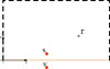 |
Figure 2. Numerical experiment setup with the image source theory. The dotted lines represent free boundaries and the orange line a perfectly reflective boundary. |
For a simulation setup as in Figure 2, with a boundary condition located at y = 0, r = ‖r − rs‖ and  become:
 (9a)
(9a)
 (9b)
(9b)
However, when these distances are discretized throughout the TLM model, special care must be taken because of the spatial discretization of the domain. Indeed, as shown in Figure 3, the distance to the boundary surface is not exactly Δxi = jiΔℓ because the meshing process introduces two artificial nodes to interface with the solver code [26]. The presence of the marker nodes (“outside” and “boundary”) leads to:
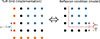 |
Figure 3. Modeling of the boundaries in the TLM implementation. Orange dots: “outside” nodes; black dots: “boundary” nodes; blue dots: “fluid” nodes. The red dotted line represents the boundary as modeled in the concept representation of Figure 1. |
 (10)
(10)
Thus, the distances of interest on the grid (noted r and r′ for clarity) are computed as:
 (11a)
(11a)
 (11b)
(11b)
Reintroducing these distances in equation (8) gives the solution for the analytical pressure on the grid  .
.
4 Numerical experiment
A numerical experiment is now carried out with the introduction of a perfectly reflective surface. The numerical results from the TLM model are compared to the image source formulation of the analytical solution described in Section 3.
4.1 Simulation setup
The numerical experiment setup displayed in Figure 4 is implemented for two main geometric parameters: the height h between the ground and the source and the maximum distance rmax between the last receiver point and the source. The number of receivers in the array is also determinant since a too-coarse matrix can lead to a lack of precision in the detection of the interference patterns. For the following experiments, a matrix of 100 ×100 receivers is used. Thus, the most important modeling parameter for the analysis is the number of points per wavelength Nppw = λ/Δℓ which is set to 10 at the maximal frequency fmax of the source emission.
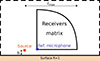 |
Figure 4. Numerical experiment setup. |
4.2 Data processing
Various approaches are available to evaluate the numerical dispersion error. In order to introduce the method, two third-order tensors  and
and  are introduced to represent numerical (TLM simulations) and analytical results respectively. They are consistent with the formalism used before (Sect. 3):
  is the pressure signal at the receiver r = (j1,j2) and at the time step n. The tensors are filled with real values that are the analytical and modeled pressure, their size is the number of time steps and the number of microphones along the two axes of the mesh.
4.2.1 Attenuation relative to a reference receiver
The SPL attenuation relative to a reference receiver is used as a metric to assess the discrepancies between simulated pressure signals and their corresponding analytical solutions. Errors are evaluated using sound attenuation levels rather than acoustic pressure to reduce sensitivity to small pressure variations that can cause disproportionate local errors, following standard practice in environmental acoustics. For every line of receivers, the reference receiver is the closest to the source. The SPL attenuation is calculated as:
 (12)
(12)
Equation (12) can also be written for  . To compare the numerical results to the analytical solutions, the following SPL absolute error is used:
![Mathematical equation: $$ \begin{aligned} \varepsilon _{j_1, j_2} = \left|A_{j_1, j_2}(\mathfrak{n} ) - A_{j_1, j_2}(\mathfrak{a} )\right| ~ [\text{ dB}]. \end{aligned} $$](/articles/aacus/full_html/2025/01/aacus240023/aacus240023-eq71.gif) (13)
(13)
For a better normalization process, a polar array of receivers is chosen to ensure that all the receivers of an arc are at the same distance from the source.
5 Results
Since the numerical dispersion affects more the high frequencies during the sound propagation [11] the analysis is performed by comparing different sources, regarding distinct spectral distributions. For a better understanding of the results, the number of points per wavelength Nppw is presented for each source. An overview of one simulation is displayed in Figure 5 for a Gaussian pulse.
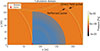 |
Figure 5. Sound pressure field for a Gaussian source at the end of the TLM simulation. The whole calculation domain is represented. At the last iteration of the calculation, reflected and incident waves have passed through all the receivers (blue dots) in the network. |
In the following subsections, the absolute errors εj1,j2 on the SPL attenuation at each receiver are displayed (cf. Eq. (13)). The objective is to determine whether dispersion-induced delayed interferences occur in the receivers’ matrix. Indeed, if there is an interference pattern for one of the delayed frequencies at a receiver, a lack of energy compared to the analytical solution will appear in the simulated signals. The following results are presented for fmax = 500 Hz, h = 2m and the sound speed c0 = 344.24 m.s−1. The simulation time is tsim = 4.19e–01 s with Δℓ = 6.88e–02 m and Δt = 4.14e–04 s. The height of the source, h is equal for all the simulations since it has been shown to affect mostly the interference patterns between the direct and reflected wavefront, leading to similar order of magnitude in the errors [14].
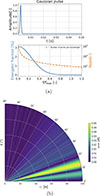 |
Figure 6. (a) Time signal according to time (top) and spectral distribution (bottom) of a Gaussian pulse compared to Nppw (orange dashed line) according to normalized frequency. (b) Polar map of the SPL absolute error εj1,j2 (Eq. (13)). |
5.1 Gaussian source
In this case, the source signal is implemented according to:
 (14)
(14)
As it can be observed in Figure 6, most of the spectral components of the Gaussian source are over-discretized and those corresponding to f ≥ fmax and Nppw ≤ 10 represent less than 2% of the signal energy. On the vertical and horizontal axes, negligible absolute errors appear between the analytical and the numerical results. In addition, an interference pattern of the error is observable with a “ray” of errors in the areas where the dispersed end of the incident wavefront interacts with its reflection.
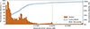 |
Figure 7. Statistical distribution of the absolute errors εj1,j2 for the Gaussian pulse case. |
In Figure 7, the statistical distribution of the SPL error is represented without considering the spatial locations. It confirms that for an over-discretized source signal, the error related to numerical dispersion is negligible (95% of the errors are below 0.03 dB).
5.2 Shifted Gaussian source
In this case, the source signal is implemented according to:
 (15)
(15)
The source has a broader spectrum than in the previous case. The excitation signal is therefore less over-sampled and the impact on the results is visible on the Figure 8b. The ray of interference also appears, but the error magnitudes are higher than for the regular Gaussian case because of the lower discretization of the source spectral components.
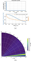 |
Figure 8. (a) Time signal according to time (top) and spectral distribution (bottom) of a shifted Gaussian pulse compared to Nppw (orange dashed line) according to normalized frequency. (b) Map of the SPL absolute error εj1,j2. |
Indeed, the maximum error is of 0.44 dB and 95% of the errors in the considered quarter circle are below 0.1 dB Figure 9. This shift of approximately a factor ten in the errors confirms that the discretization of the modeled wave packet influences the numerical dispersion effect on long-range results (rmax ≈ 150 × λmin here).
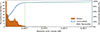 |
Figure 9. Statistical distribution of the absolute errors εj1,j2 for the shifted Gaussian pulse case. |
5.3 Windowed sinusoidal source
In this case, the source signal is implemented according to:
![Mathematical equation: $$ \begin{aligned} \sin _\text{ w}[n] = \text{ w}_\text{ hann} \times \sin \left( 2 \pi f_\text{ max} n \mathrm{\Delta } t \right) \end{aligned} $$](/articles/aacus/full_html/2025/01/aacus240023/aacus240023-eq95.gif) (16)
(16)
with Whann a Hann window of duration 0.15 × tsim. The two previous cases implied broadband sources. Now, a windowed sine is used as it is pseudo-harmonic. As shown in Figure 10a, most of the source energy is focused around the frequency fmax and has a 10-point spatial discretization. Thus, the direct wave is more likely to interfere with the reflected one. With this spectral distribution, significant interference-induced errors are generated by the numerical dispersion (up to 11.06 dB as shown in Fig. 10b). Indeed, at some receivers, the energy of the received signal is either increased or lost due to artificial interference patterns induced by the TLM model. Comparing Figures 10b, 8b and 6b also leads to the conclusion that the spectral distribution of the source has an impact on the spatial distribution of the error: the wider the spectral distribution of the source is, the wider the spatial distribution of the error.
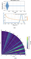 |
Figure 10. (a) Time signal according to time (top) and spectral distribution (bottom) of a windowed sine compared to Nppw (orange dashed line) according to normalized frequency. (b) Polar map of the SPL absolute error εj1,j2 (Eq. (13)). |
In this case, the histogram in Figure 11 presents a broader occurrence distribution of the errors compared to Figures 7 and 9. The most critical value is that 5% of the errors are in the interval [5–11 dB]. This value suggests that depending on the source definition, more than ten points per wavelength are needed to model the propagation of wave packets with the TLM model. To make the concept of misplaced interference patterns clearer, the next Section 5.4 shows in more detail the attenuation along receiver lines of interest.
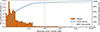 |
Figure 11. Statistical distribution of the absolute errors εj1,j2 for the windowed sine case. |
5.4 Attenuation along line
To better explain the maxima of errors presented in the windowed sine case, Figure 12 displays the SPL attenuation relative to the reference receiver for three lines of receivers: θ = [4°, 10°, 15°]. The plots in Figure 12 help visualize better the lines of receivers on the previous color maps.
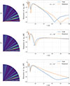 |
Figure 12. Numerical SPL attenuation relative to a reference receiver according to the propagation distance r (blue line), compared to the analytical solution (orange dashed line) for three source-receiver angles: (a) θ = 4°, (b) θ = 10° and (c) θ = 15°. Source located at hs = 2m and emitting a windowed sinusoidal signal at fmax = 500 Hz (Nppw = 10). On the error maps on the left, red lines indicate the receiver lines corresponding to the SPL attenuation graphs on the right. |
The “Sawtooth” effect on the attenuation profiles comes from the Cartesian discretization of the numerical domain. It does not affect the results as it is present for both analytical and numerical solutions. In Figure 12a and 12c related to θ = 4° and θ = 15°, it is observed that maxima of errors are due to misplacement of attenuation peaks along the source-receiver distance. The θ = 15° line is the one that presents the largest gap because the third attenuation peak is simulated closer to the source than the analytical solution.
6 Comparison to FDTD schemes
Since the FDTD is the closest numerical method to the TLM in terms of discretization of partial differential equations, it seems relevant to compare the error on the modeled axial sound speeds from the two models. As highlighted by the stability analysis of the TLM model, the numerical dispersion is maximal along the main directions of the mesh [11]. Thus, considering θ the angle between the plane wave vector and the horizontal direction of the mesh, the numerical phase speed in a 2D Cartesian grid cph can be expressed as a function of Nppw on the main directions of the mesh ( ,
,  ), as
), as
![Mathematical equation: $$ \begin{aligned} c_\text{ ph} = c~\frac{N}{\pi \sqrt{2}} \arccos \left[ \frac{1}{2} \left(\cos \left(\frac{2 \pi }{N_\text{ ppw}}\right) + 1\right)\right], \end{aligned} $$](/articles/aacus/full_html/2025/01/aacus240023/aacus240023-eq120.gif) (17)
(17)
with c the modeled sound speed in the propagation medium.
Similar expressions can be formulated for the group speed, for 3D cases or other “Taylor-expansions series based” numerical methods [16]. In Figure 13, the phase and group speeds associated with centered finite difference schemes are compared to the ones related to the TLM method. From these figures, it is straightforward that increasing the method order reduces the dispersion errors and that the phenomenon is stronger on the group speed. For instance, more than 30 points per wavelength would be needed for the TLM to get the accuracy that the fourth-order FDTD scheme has at N = 10.
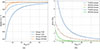 |
Figure 13. (a) Effective speeds compared to the physical constant; (b) Relative errors on the phase and group velocities [%] related to the model anisotropy depending on the number Nppw. “DFOD2” and “DFOD4” stand for the second and fourth-order centered finite difference schemes, respectively. |
As mentioned in Section 2, it is straightforward on Figure 13b that the TLM and the second-order FDTD numerical phase speeds are completely equivalents. Hence, the same conclusion is applied to the numerical group speed. Additionally, Figure 13b shows that the same number of points per wavelength would result in the same dispersion error for the two methods, so the numerical cost of using the TLM or a second order FDTD is the same. The comparison results with fourth-order FDTD confirm that for in-volume modeling, the TLM method is not the most performant method for universal applications. However, this statement can be moderated by the fact that a lower-order scheme implies less implementation complexity on the boundary conditions. Thus, when numerous scatterers are considered, second-order schemes could be attractive for their computational costs.
7 Conclusion
The limitations of the TLM model for long-range sound propagation simulations over a rigid ground were investigated thanks to numerical experiments and a theoretical comparison. A polar array of virtual receivers has been used to study the interactions between simulated direct sound waves and their reflection. The results from three distinct source signals emphasize the importance of the number of points per wavelength as a simulation parameter. The presence of a perfect specular reflection in the model shows that numerical dispersion can affect the simulated sound pressure levels. In specific cases of reflection, misplaced simulated interferences appear due to the wrongly approximated group speed of some spectral components of the wave packet. Relatedly, the link between the spatial distribution of the errors and the spectral distribution of the source has been highlighted. Finally, a comparison between the TLM model and a higher-order centered FDTD method stated that for general in-volume modeling, the TLM is not the more efficient method against numerical dispersion as it requires a finer discretization of the mesh.
However, since a higher-order spatial integration requires a higher-order integration scheme for the boundary conditions, the idea of using a low-order scheme to model a complex environment needs further analysis. In addition, the use of a non-dissipative method such as TLM in multiple scatterers and source scenarios where the dispersion-induced error could be mitigated seems to be a promising and computationally efficient approach. A comparison with in-situ measurements under real outdoor conditions should be made to characterize the reliability of the simulated sound pressure levels in environmental acoustics applied cases. In addition, further research to increase the accuracy of the TLM model from second to fourth order could help in the effort to compare its performance with finite difference schemes.
Acknowledgments
The authors would like to acknowledge the High Performance Computing Center of the University of Strasbourg for supporting this work by providing scientific support and access to computing resources. Part of the computing resources were funded by the Equipex Equip@Meso project (Programme Investissements d’Avenir) and the CPER Alsacalcul/Big Data.
Conflicts of interest
The authors declare no conflicts of interest.
Data availability statement
Data are available on request from the authors.
References
- WHO: Environmental Noise Guidelines for European Region. WHO Regional Office for Europe, Copenhagen, 2019. [Google Scholar]
- G. Dutilleux: Anthropogenic sound and terrestrial ecosystems: a review of recent evidence, in: Proceedings of 12th ICBEN Congress on Noise as a Public Health Problem, Zürich, Switzerland, 2017. [Google Scholar]
- R. Sordello, O. Ratel, F. Flamerie De Lachapelle, C. Leger, A. Dambry, S. Vanpeene: Evidence of the impact of noise pollution on biodiversity: a systematic map. Environmental Evidence 9, 1 (2020) 20. [Google Scholar]
- S. Haupert, F. Sèbe, J. Sueur: Physics-based model to predict the acoustic detection distance of terrestrial autonomous recording units over the diel cycle and across seasons: insights from an alpine and a neotropical forest. Methods in Ecology and Evolution 14, 2 (2023) 614–630. [Google Scholar]
- European Commission. Joint Research Centre. ICHP: Common Noise Assessment Methods in Europe (CNOSSOS-EU): to be used by the EU member states for strategic noise mapping following adoption as specified in the environmental noise directive 2002/49/EC. Publications Office, LU, 2012. [Google Scholar]
- M. Kaltenbacher, ed.: Computational Acoustics. Vol. 579 of CISM International Centre for Mechanical Sciences. Springer International Publishing, Cham, 2018, DOI: http://dx.doi.org/10.1007/978-3-319-59038-7. [Google Scholar]
- G.C. Cohen: Higher-Order Numerical Methods for Transient Wave Equations. Vol. 110 of Scientific Computation. Springer Berlin Heidelberg, Berlin, Heidelberg, 2002. [Google Scholar]
- E.M. Salomons: Computational Atmospheric Acoustics. Springer Netherlands, Dordrecht, 2001. [Google Scholar]
- M. Hornikx: Ten questions concerning computational urban acoustics. Building and Environment 106 (2016) 409–421. [Google Scholar]
- G. Guillaume, N. Fortin: Optimized transmission line matrix model implementation for graphics processing units computing in built-up environment. Journal of Building Performance Simulation 7, 6 (2014) 445–456. [Google Scholar]
- Q. Goestchel, G. Guillaume, D. Ecotière, B. Gauvreau: Analysis of the numerical properties of the transmission line matrix model for outdoor sound propagation. Journal of Sound and Vibration 531 (2022) 116974. [Google Scholar]
- P. Aumond, G. Guillaume, B. Gauvreau, C. Lac, V. Masson, M. Bérengier: Application of the transmission line matrix method for outdoor sound propagation modelling – part 2: experimental validation using meteorological data derived from the meso-scale model Meso-NH, Applied Acoustics 76 (2014) 107–112. [Google Scholar]
- P. Chobeau, G. Guillaume, J. Picaut, D. Ecotière, G. Dutilleux: A transmission line matrix model for sound propagation in arrays of cylinders normal to an impedance plane. Journal of Sound and Vibration 389 (2017) 454–467. [Google Scholar]
- Q. Goestchel: Acoustic propagation in forest environments: time domain numerical methods toward bioacoustic applications. PhD thesis, Le Mans Université, 2023. https://theses.hal.science/tel-04357383. [Google Scholar]
- G.C. Cohen: Numerical Dispersion and Anisotropy, in: G.C. Cohen, ed. Higher-Order Numerical Methods for Transient Wave Equations, Scientific Computation, Springer, Berlin, Heidelberg, 2022, pp. 101–121. [Google Scholar]
- L.N. Trefethen: Group velocity in finite difference schemes. SIAM Review 24, 2 (1982) 113–136. [CrossRef] [Google Scholar]
- C. Bogey, C. Bailly: A family of low dispersive and low dissipative explicit schemes for flow and noise computations. Journal of Computational Physics 194, 1 (2004) 194–214. [CrossRef] [Google Scholar]
- C. Bailly, C. Bogey: An overview of numerical methods for acoustic wave propagation, in: European Conference on Computational Fluid Dynamics, 2006. [Google Scholar]
- L. Savioja, V. Valimaki: Reducing the dispersion error in the digital waveguide mesh using interpolation and frequency-warping techniques. IEEE Transactions on Speech and Audio Processing 8, 2 (2000) 184–194. [Google Scholar]
- G. Campos, D. Howard: On the computational efficiency of different waveguide mesh topologies for room acoustic simulation. IEEE Transactions on Speech and Audio Processing 13, 5 (2005) 1063–1072. [Google Scholar]
- Y. Kagawa, T. Tsuchiya, B. Fujii, K. Fujioka: Discrete Huygen’s model approach to sound wave propagation. Journal of Sound and Vibration 218, 3 (1998) 419–444. [Google Scholar]
- G. Guillaume, J. Picaut, G. Dutilleux, B. Gauvreau: Time-domain impedance formulation for transmission line matrix modelling of outdoor sound propagation. Journal of Sound and Vibration 330 (26) (2011) 6467–6481. [Google Scholar]
- M. Bruneau, Fundamentals of Acoustics. ISTE Ltd, London; Newport Beach, CA, 2006. [Google Scholar]
- W. Duan, R. Kirby: The sound power output of a monopole source in a cylindrical pipe containing area discontinuities, in: Proceedings of Acoustics 2012, Nantes, France, 7, 2012. [Google Scholar]
- I. Rudnick: The propagation of an acoustic wave along a boundary. The Journal of the Acoustical Society of America 19, 2 (1947) 348–356. [Google Scholar]
- G. Guillaume, N. Fortin, B. Gauvreau, J. Picaut: TLM OpenCL: multi-GPUs implementation to cite this version: HAL Id: Hal-00804170, 2013, pp. 3249–3255.https://hal.science/hal-00804170/. [Google Scholar]
Cite this article as: Goestchel Q. Guillaume G. Ecotière D. & Gauvreau B. 2025. Transmission line matrix model: numerical dispersion effects on simulated specular reflection. Acta Acustica, 9, 72. https://doi.org/10.1051/aacus/2025057.
All Figures
|
Figure 1. Representation of the 2D simple boundary reflection at the local node r = (j1, j2) close to a boundary of reflection coefficient R1. On the line m = 1, scattered pulse “S” (orange) at time step n becomes a reflected incident pulse “I” (blue) at next step n+1. |
| In the text | |
|
Figure 2. Numerical experiment setup with the image source theory. The dotted lines represent free boundaries and the orange line a perfectly reflective boundary. |
| In the text | |
|
Figure 3. Modeling of the boundaries in the TLM implementation. Orange dots: “outside” nodes; black dots: “boundary” nodes; blue dots: “fluid” nodes. The red dotted line represents the boundary as modeled in the concept representation of Figure 1. |
| In the text | |
|
Figure 4. Numerical experiment setup. |
| In the text | |
|
Figure 5. Sound pressure field for a Gaussian source at the end of the TLM simulation. The whole calculation domain is represented. At the last iteration of the calculation, reflected and incident waves have passed through all the receivers (blue dots) in the network. |
| In the text | |
|
Figure 6. (a) Time signal according to time (top) and spectral distribution (bottom) of a Gaussian pulse compared to Nppw (orange dashed line) according to normalized frequency. (b) Polar map of the SPL absolute error εj1,j2 (Eq. (13)). |
| In the text | |
|
Figure 7. Statistical distribution of the absolute errors εj1,j2 for the Gaussian pulse case. |
| In the text | |
|
Figure 8. (a) Time signal according to time (top) and spectral distribution (bottom) of a shifted Gaussian pulse compared to Nppw (orange dashed line) according to normalized frequency. (b) Map of the SPL absolute error εj1,j2. |
| In the text | |
|
Figure 9. Statistical distribution of the absolute errors εj1,j2 for the shifted Gaussian pulse case. |
| In the text | |
|
Figure 10. (a) Time signal according to time (top) and spectral distribution (bottom) of a windowed sine compared to Nppw (orange dashed line) according to normalized frequency. (b) Polar map of the SPL absolute error εj1,j2 (Eq. (13)). |
| In the text | |
|
Figure 11. Statistical distribution of the absolute errors εj1,j2 for the windowed sine case. |
| In the text | |
|
Figure 12. Numerical SPL attenuation relative to a reference receiver according to the propagation distance r (blue line), compared to the analytical solution (orange dashed line) for three source-receiver angles: (a) θ = 4°, (b) θ = 10° and (c) θ = 15°. Source located at hs = 2m and emitting a windowed sinusoidal signal at fmax = 500 Hz (Nppw = 10). On the error maps on the left, red lines indicate the receiver lines corresponding to the SPL attenuation graphs on the right. |
| In the text | |
|
Figure 13. (a) Effective speeds compared to the physical constant; (b) Relative errors on the phase and group velocities [%] related to the model anisotropy depending on the number Nppw. “DFOD2” and “DFOD4” stand for the second and fourth-order centered finite difference schemes, respectively. |
| In the text | |
Current usage metrics show cumulative count of Article Views (full-text article views including HTML views, PDF and ePub downloads, according to the available data) and Abstracts Views on Vision4Press platform.
Data correspond to usage on the plateform after 2015. The current usage metrics is available 48-96 hours after online publication and is updated daily on week days.
Initial download of the metrics may take a while.