| Issue |
Acta Acust.
Volume 10, 2026
|
|
|---|---|---|
| Article Number | 5 | |
| Number of page(s) | 16 | |
| Section | Computational and Numerical Acoustics | |
| DOI | https://doi.org/10.1051/aacus/2025071 | |
| Published online | 13 February 2026 | |
Scientific Article
How elevated sources can cause local increases of sound pressure levels in the upwind domain
Deutsches Zentrum für Luft- und Raumfahrt, Institut für Physik der Atmosphäre, Oberpfaffenhofen Germany
* Corresponding author: This email address is being protected from spambots. You need JavaScript enabled to view it.
Received:
15
May
2025
Accepted:
7
December
2025
Abstract
While increased sound levels near the ground in downwind conditions are a well-studied topic, comparatively little attention has been given in the literature to increased sound pressure levels in upwind propagation. This increase, however, typically occurs only under specific conditions, including an elevated source location, a non-linear (e.g., logarithmic) wind or temperature profile, and a focus on particular distances within the upwind domain. These conditions are known to be responsible for the formation of caustics. Simultaneously, the sound level enhancement may be disturbed by diffraction, ground reflection, and its characteristics depend on the source structure, being most readily derivable for point sources. Consequently, investigations using models and comparisons with observations are challenging. This work uses two fundamentally different modelling approaches in their ability to capture such phenomena. The goal is to provide an intuitive understanding of the complex interactions involved in sound propagation under real atmospheric conditions, thereby supporting the interpretation of acoustic simulation and measurements in applied contexts.
Key words: Sound propagation simulation / Wind energy / Refraction / Outdoor sound propagation / Elevated sources
© The Author(s), Published by EDP Sciences, 2026
 This is an Open Access article distributed under the terms of the Creative Commons Attribution License (https://creativecommons.org/licenses/by/4.0), which permits unrestricted use, distribution, and reproduction in any medium, provided the original work is properly cited.
1 Introduction
The effect of increased sound levels in downwind conditions has long been known and is widely accepted. The physical mechanism behind this phenomenon includes the downward refraction of sound waves in a stratified medium and multiple reflections off the ground. Temperature inversions or downwind conditions can sometimes create a near-ground sound duct, allowing sound to propagate over long distances with minimal attenuation [1, 2].
In contrast, upwind conditions or unstable temperature stratification lead to upward refraction, eventually resulting in pronounced sound shadow zones at a certain distance, where signals from the source are significantly attenuated or even undetectable (e.g., [3, 4]). As a result, a widely held assumption is that sound pressure levels (SPL) observed in the upwind region remain comparatively lower than those observed downwind (e.g., [5, 6]).
When investigating noise from elevated sound sources, such as wind turbines, departing and landing aircraft, or the sonic boom, sometimes references can be found in the literature to increased sound levels in upwind conditions (e.g.: wind turbine noise: [7, 8], sonic boom: [9] or aircraft noise: [10]). All four studies, either show caustics/sound level increases in upwind conditions without delving deeper into the physical explanation, or the fourth one shows graphical representations of sound rays and their connection to caustics. The studies by Heimann et al. [11], Cotté et al. [7], and Colas et al. [8] model sound propagation from wind turbines under different atmospheric conditions. The figures presented in these studies reveal that, in certain scenarios, there is an increase in sound pressure levels in the upwind direction. In [12], the possible creation of noise reinforcement zones in the upwind domain have been described, but with a focus on the interaction of two wind turbines.
However, increased sound levels are sometimes observed and are a cause of complaints in upwind regions from wind turbines may be a result of caustics, if the right combination of conditions is met, particularly near the shadow boundary. In [13], caustics are described in basic terms, and their formation in the upwind direction due to sound focusing is explained, though the link to practical applications is not strongly emphasized.
High sound pressure levels in the upwind domain can be found, at elevated sound sources in combination with special meteorological situations on far field sound propagation, in spatially limited regions (i.e., specific distances from the source and specific measurement heights above ground). So, special geometric setups might be one reason why studies that combine simulations with measurements of sound pressure levels remain scarce. Another reason for this lack of attention may be that the effect becomes noticeable only under specific conditions such as elevated sources combined with logarithmic (i.e., non-linear) upward refraction. Additionally, the source should be “sharp”, for example a point source, and other interfering effects such as turbulence or ground reflections should be minimized. These latter factors again especially impair the detectability of this phenomenon in measurements.
On the modelling side, many approaches especially engineering schemes that account for upwind/downwind conditions or temperature gradients rely on linear profiles of wind and temperature. As a result, this effect cannot be reproduced by such models.
Therefore the aim of this paper is to carefully evaluate the simulation results and demonstrate the origin of the effect of sound level increase in the upwind domain. In order to achieve this, simulations with different setups have been performed using a particle-based model. Here, the influence of several sound propagation effects on the respective results has been analysed. The particle-based model helps in the intuitive visualization of the propagation paths and the effects are easy to understand. To exclude a model specific behaviour, the results have been backed up by a wave-based finite difference time domain (FDTD) sound propagation model. The FDTD model with its direct solution of the wave equation simulates all wave phenomena physically correctly and is very well suited for complex, inhomogeneous media, but requires significantly more computational power. This dual-model strategy enables us to distinguish the physical effects. A recent code-to-code comparison in wind energy applications by Elsen et al. [14] further demonstrates the value of combining different modelling techniques to validate and interpret simulation results. Therefore, Section 2 gives a brief overview on the sound propagation models involved in this study, Akumet and Aku3d. The setup and first results are introduced in Section 3. Section 4 concentrates on the analysis and explanation of the origin of the increased sound pressure level in the upwind domain by reducing the domain to two dimensions (Sect. 4.1), analysing different refractive conditions (Sect. 4.2) and finally comparing the results to the wave based model Aku3d (Sect. 5). A summary of our findings is given in Section 6.
2 Overview on the sound propagation models
This study uses two fundamentally different modelling approaches with distinct advantages in their ability to capture and explain the effect of caustics due to refraction, as well as many other physical effects influencing the sound pressure field in long-range sound propagation.
2.1 Particle-based model (Akumet)
The particle-based, Lagrangian model Akumet as described by Heimann et al. [15], models sound propagation by distributing sound energy among a given number of sound particles and tracking their paths through the atmosphere. This approach is based on geometrical acoustics, which is a simplification of the wave equation under the assumption of high frequencies and short wavelengths compared to object sizes. The particle paths describe the direction of the wavefront’s propagation or in other words, the normal vector to the wavefront itself. The model was designed specifically for simulating long range sound propagation over hilly terrain in an inhomogeneous atmosphere.
Therefore, a frequency-dependent fraction of the sound pressure amplitude:
 (1)
(1)
is assigned to each particle j (j = 1, …, N), where ρs and cs are the air density and sound speed at the source, respectively. The sound intensity J0(f) at a distance s0 from the source is given by:
 (2)
(2)
where P s (f) is the frequency-specific sound power and Δψ the radiation sector. Depending on the source type, a 1 is set to 2 for a point source or 1 for a line source.
The path of each particle is represented by a ray vector  and a unit vector
  , normal to the wavefront. These vectors are governed by differential equations from Pierce et al. [16]:
 (3)
(3)
 (4)
(4)
where  is the speed of sound;
  is the three-dimensional wind vector, κ = c
p
/c
v
= 1.402 is the ratio of specific heat capacities, R
L
= 287.058 J/kgK is the gas constant for dry air and T is the air temperature in Kelvin. Equations (3) and (4) are numerically integrated for all particles using forward-time integration until they exit the computational domain. This means that each time step t each particle that was released from the source is tracked along its propagation path, which are stored in a list of (x, y, z)-coordinates. This path is also denoted as ray and each coordinate (x
t
, y
t
, z
t
) is denoted as particle position. At the end of the simulation, a sound pressure level is computed based on particles passing through so-called control volumes of a given size, i.e., the number of particle positions in each of these volumes. The model considers different ground conditions, air absorption, refraction, diffraction close to the ground, interference and arbitrary-shaped obstacles. Meteorological data, such as wind speed and temperature distribution, are supplied by a flow model, enabling realistic terrain and atmospheric effects.
is the three-dimensional wind vector, κ = c
p
/c
v
= 1.402 is the ratio of specific heat capacities, R
L
= 287.058 J/kgK is the gas constant for dry air and T is the air temperature in Kelvin. Equations (3) and (4) are numerically integrated for all particles using forward-time integration until they exit the computational domain. This means that each time step t each particle that was released from the source is tracked along its propagation path, which are stored in a list of (x, y, z)-coordinates. This path is also denoted as ray and each coordinate (x
t
, y
t
, z
t
) is denoted as particle position. At the end of the simulation, a sound pressure level is computed based on particles passing through so-called control volumes of a given size, i.e., the number of particle positions in each of these volumes. The model considers different ground conditions, air absorption, refraction, diffraction close to the ground, interference and arbitrary-shaped obstacles. Meteorological data, such as wind speed and temperature distribution, are supplied by a flow model, enabling realistic terrain and atmospheric effects.
Heimann et al. [15] validated Akumet through comparisons with analytical solutions and benchmark data from fast-field-program models. Its reliability has been demonstrated in works such as Blumrich et al. [17], Heimann et al. [11, 18], and Kästner et al. [19]. In addition, Akumet was used by Gharbi et al. [20] to reconstruct overflights of a small aircraft, considering local meteorological conditions, and to compare the simulations with the measurement campaign. The simulation results presented in [20] show good agreement with the measurement data in [21].
While Akumet efficiently tracks sound energy via discrete particle trajectories [15], making it particularly suitable for long-range sound propagation simulations, it does not fully capture all wave phenomena, like for example diffraction around obstacles. Therefore, the wave-based model Aku3d was used in order to complement the results obtained using Akumet and verify the observed effects.
2.2 FDTD-Model (Aku3d)
The wave-based FDTD model Aku3d as described by Blumrich et al. [22] and Heimann et al. [23], is based on the governing equations for a compressible and adiabatic gaseous medium in a non-rotating system. The model relies on the equation of motion, the continuity equation, and the first law of thermodynamics for adiabatic processes. This model can simulate all wave phenomena such as reflection, refraction, diffraction, interference, and scattering physically correctly. The atmospheric state variables ϕ = (u, p, ρ) are split into meteorological, turbulent, and acoustic components:
 (5)
(5)
where  denotes the mean atmospheric state, a single prime (ϕ′) indicates the turbulent deviations from the mean meteorological values, and the double prime (ϕ′′) describes the deviations from the mean field according to acoustic waves (in particular sound pressure p′′ and particle velocity u
′
′). The model solves the prognostic equations for u
′
′ and p′′ by substituting
denotes the mean atmospheric state, a single prime (ϕ′) indicates the turbulent deviations from the mean meteorological values, and the double prime (ϕ′′) describes the deviations from the mean field according to acoustic waves (in particular sound pressure p′′ and particle velocity u
′
′). The model solves the prognostic equations for u
′
′ and p′′ by substituting  and
and  . The equations are then linearized with respect to the mean meteorological state, with turbulent components disregarded due to the assumption of a stationary atmosphere.
A diffusion term is added to account for atmospheric absorption, simulating energy loss during sound propagation. ν denotes the kinematic viscosity coefficient, introduced to account for dissipative effects such as viscous damping. Gravity is neglected, resulting in:
 (6)
(6)
 (7)
(7)
 (8)
(8)
The resulting equations are solved numerically on an orthogonal staggered grid with the explicit forward-in-time RK3-scheme. The full derivation of the equations can be found in [22].
Aku3d integrates meteorological data from external flow models that provide the spatial distribution of atmospheric fields such as wind velocity, temperature gradients, and density. These fields, denoted as u met, p met, and ρ met, serve as input in order to simulate sound propagation under realistic atmospheric conditions. This data directly influences the propagation of sound waves by affecting factors such as refraction and changes in the speed of sound. Aku3d assumes a “frozen” atmosphere, meaning that these fields remain stationary during the sound propagation simulation. At open boundaries Aku3d applies the scheme for perfectly matched layers (PML) [24]. On the ground the scheme according to Heutschi et al. [25] is implemented.
In Aku3d the sound source can either be defined as a harmonic pressure source at a single point or as a Gaussian pulse with a certain spatial extension. In case of a harmonic pressure source, the sound pressure at a single grid cell (x s , y s ) is defined as follows:
 (9)
(9)
where p i is the pressure amplitude at frequency f i . In order to initialize a broadband sound pressure wave a spatial distributed Gaussian pressure pulse, can be defined as follows:
 (10)
(10)
with s the spatial variable (here length in meter). A is the amplitude of the pressure pulse and σ s is the standard deviation (related to the pulse width in space), defined in Aku3d through the FWHM of the Gaussian pulse:
 (11)
(11)
The corresponding frequency domain width can be determined by transforming the spatial extension into a temporal distribution and then applying a Fast Fourier Transformation on equation (10).
Since the Fourier transform of a Gaussian is Gaussian, the frequency domain source spectrum G(f) of a spatial Gaussian pulse define above with width σs (from the FWHM) is given by Dragna et al. [26]:
![Mathematical equation: $$ \begin{aligned} G(f)=A\,\frac{i\,2\pi f}{c_0}\,\left(\sqrt{2\pi }\,\sigma _s\right)^{n} \exp \!\left[-2\left(\frac{\pi f\,\sigma _s}{c_0}\right)^2\right], \end{aligned} $$](/articles/aacus/full_html/2026/01/aacus250062/aacus250062-eq21.gif) (12)
(12)
where A is an amplitude factor, c0 is the sound speed, and n = 2 (2D) or n = 3 (3D). Decreasing σs shifts to higher f, motivating a conservative choice of fmax (and thus grid spacing).
3 Initial problem from practical findings
Within this section we present the occurrence of caustics in our model setup, that might occur in wind energy application. Especially the difference between an elevated source represented as a point source in contrast to a spatially distributed source. First, detailed information on the simulation setups are provided. All simulations within this section have been performed using the particle-based model Akumet.
3.1 Simulation setup
The first test case was characterised by a flat topography and a simple meteorological profile, with the computational domain being defined as x : [ − 1000, 1000] m, y : [ − 800, 800] m, z : [0, 248] m.
The spatial resolution of the evaluation domain is 8 m in all three dimensions, i.e., the simulated sound pressure levels are averaged over control volumes of 8 × 8 × 8 m, meaning that the average height  of the k-th control volume above ground is
 (13)
(13)
where K is the total number of cells in the z-direction. In the following, this average height will be referred to in order to address a specific control volume, e.g., speaking of a height of 4 m above ground refers to the control volume that ranges from 0 m to 8 m above ground. According to the Delany–Bazley and to Miki [27, 28], the ground conditions were set to complex impedance with a ground resistivity of 300.0 kPa/m2s.
The source (here: wind turbine) is located at (x 0, y 0)=(0, 0) with a source height (hub) of 100 m and a rotor diameter of 80 m. In case 1a, the source is defined as a simple point source while in case 1b it is defined using 36 point sources, placed in a circle of the same diameter as the rotor in order to consider the rotational character of the source (as indicated by the red dots in Fig. 1). A similar setup has for example been used in [11, 29]. In both cases the total sound power level is 107 dB. The frequency spectrum is applied for all 1/3 octave bands from 20 Hz to 16 kHz and the distribution of the sound power level across all frequencies is according to [30]. The source is defined as incoherent, while source directivity is not accounted for.
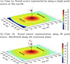 |
Figure 1. Simulated sound pressure level at ground level (4 m above ground) for test case 1. The increased sound levels in the upwind domain are clearly visible for both source setups, but more pronounced for the single point source setup (a). (a) Case 1a: Sound source representation using a single point source at the nacelle. (b) Case 1b: Sound source representation using 36 point sources, distributed along the rotational plane. |
The meteorological profiles were assumed to be constant horizontally (x, y) and thus only vary with z. To retrieve the logarithmic wind profile as used in the sound propagation codes Akumet and Aku3d, given a roughness length z 0, the wind speed u(z) for any given height z is calculated from the reference height z r and reference wind speed u r as follows:
 (14)
(14)
The logarithmic wind profile was calculated for z 0 = 0.2 m, z r = 10 m and u r = 5 m/s, the wind direction was defined as 270°, i.e., the wind is blowing in positive x-direction. Therefore, distances measured in x-direction, i.e., following the wind direction, will also be referred to as longitudinal distance whereas distances measured in y-direction will be referred to as lateral distance (see Fig. 1).
Simulations were performed for a ground temperature of 20 °C and an isothermal temperature profile (dT/dz = 0). Air absorption was calculated according to ISO 9613-1 [31]. The general setup for test cases 1a and 1b is summarized in Table 1.
Basic setup for case 1.
3.2 Simulation results
Figure 1 shows the simulated sound pressure levels at the bottom-most level (i.e., on average 4 m above ground) for test cases 1a (single source) and 1b (multiple sources). In both cases an increased sound pressure level in the upwind domain compared to the downwind domain can be observed.
More specifically, in test case 1a (see Fig. 1a), the formation of a shadow-zone in the upwind domain is clearly visible at the left border of the computational domain at a radial distance of about 1000 m. However, there is also a strong increase in sound pressure level directly before the beginning of the shadow zone, appearing as a wave-like structure.
In test case 1b (see Fig. 1b), no formation of a shadow zone is found within the range of the computational domain. Instead, the results show a significant increase in sound pressure level in the upwind domain compared to the downwind domain. In contrast to case 1a, the above described formation of a wave-like structure cannot be observed, at least in the layer shown here. Towards the boundary of the domain the sound pressure level in the upwind domain quickly drops and becomes lower than in the respective downwind domain.
3.3 Analysis and discussion
In order to get a better picture of the sound pressure level fields, the vertical cross sections of test cases 1, are shown in Figure 2. One can clearly see the increased sound pressure levels in the upwind domain. Furthermore, in case 1a (single source, Fig. 2a) the occurrence of interference-like patterns can be observed. They are particularly pronounced, in the upwind domain but are present in the downwind domain as well.
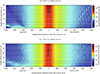 |
Figure 2. Vertical cross section of the sound pressure level field through the wind turbine (y = 0), shown for the lowest 80 m. The 4 black dashed lines indicate the mean heights of the sound pressure level curves shown in Figure 3. (a) Case 1a (single source). (b) Case 1b (multi-source). |
The seemingly higher sound emission level in case 1a (single source, Fig. 2a) compared to case 1b (multi-source, Fig. 2b) results from the multiple point source layout in case 1b. In that cross section, only two of the 36 sources are visible, and only one is shown, since the vertical domain is cut off at z = 80 m. In case 1a instead, the sound source is defined as single point source and the depicted cross section cuts right through it. A direct comparison of the sound pressure levels at four different heights (4 m, 12 m, 20 m and 76 m (hub height)) is shown in Figure 3. For reference, these four heights are also indicated by black dashed lines in Figure 2. In the following, the sound pressure level fields along these four different height levels shall be described more in detail. For test case 1a (single source, Fig. 3a) one finds at:
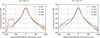 |
Figure 3. Sound pressure levels through y = 0 for selected heights (4 m, 12 m, 20 m and 76 m) above ground as indicated by the black dotted lines in Figure 2. (a) Case 1a. (b) Case 1b. |
4 m: apart from the shadow zone the sound pressure level in the upwind domain is higher compared to the downwind domain. In the upwind domain a significant increase in sound pressure level of about 3 dB is found. It is preceded by a small drop in sound pressure level, at the same distance from the source where the formation of an interference pattern in Figure 3a can be observed.
12 m: the findings are very similar to the previous layer (4 m), however, the increase of sound pressure level in the upwind domain occurs later on, i.e., at a larger distance from the source.
20 m: the sound pressure level in the upwind domain is now lower than in downwind domain. At about –700 m a local drop in sound pressure level in the upwind domain, followed by a rise in sound pressure level at about 950 m upwind of the source can be observed.
76 m: the sound pressure level in the upwind domain is lower than in the downwind domain. The downwind domain shows oscillations in the sound pressure level that are caused by the low particle density towards the boundary of the domain.
For test case 1b (multi source, Fig. 3b) one finds at:
4 m: the increase in sound pressure level is more extended with an earlier onset compared to the single source case. This can be explained by the vertical distribution of the sources: the sources situated lower to the ground lead to the earlier onset while the sources above hub height postpone the onset of the shadow zone.
12 m & 20 m: up to about –600 m in case of the 12 m layer and –750 m in the 20 m layer, the sound pressure level in the upwind domain is lower than in the respective downwind domain. Further upwind the sound pressure levels increase significantly and get about 4 dB higher than in downwind conditions before decreasing again.
76 m: for hub height, no increase upwind can be observed within the computational domain. Within a range of 1000 m from the source, the SPL downward is always higher compared to upward.
Figure 4 highlights the absolute differences in sound pressure level between upwind and downwind. For the single source (case 1a, Fig. 4a), these differences close to the ground reach a maximum of nearly 10 dB, at a distance of slightly above 800 m upwind of the source. The sound pressure level in the upwind domain clearly starts to exceed to downwind levels at a distance of about 550 m from the source and falls below the downwind levels at a distance of about 940 m from the source. In case of the distributed source (case 1b, Fig. 4b), the sound pressure levels close to the ground in the upwind domain start exceeding the downwind levels at a distance of about 350 m from the source, reaching a maximum of about 4 dB at distances between 600 m and 800 m upwind of the source. Within the computational domain, the upwind sound pressure levels do not fall below the downwind levels, where at a distance of 1000 m from the source, the upwind sound levels are still ∼2 dB higher than the downwind ones. Both, the less sharp increase of the differences in sound pressure level, as well as the wider longitudinal spread in case 1b compared to case 1a is caused by the spatial distribution of the source, as the single source is more focused compared to the multi source.
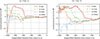 |
Figure 4. Differences in sound pressure levels between upwind and downwind, through y = 0 for selected heights (4 m, 12 m, 20 m and 100 m) above ground as indicated by the black dotted lines in Figure 2. (a) Case 1a. (b) Case 1b. |
4 Theoretical approach
The goal of the next three test cases is to explain the mechanisms involved in the effect of caustics (test case 2, Sect. 4.1), analysing the effect of different refractive conditions (Sect. 4.2) and verifying the reproducibility of the effect using a second sound propagation model (Aku3d Sect. 5). Note that throughout the paper, sound pressure levels resulting from simulations using frequency spectra are always given in dB(A) whereas for single frequency simulations dB is used.
4.1 Test case 2 – Reduction to 2D
To narrow down the problem, the setup was first reduced to the 2D-domain. To eliminate ground reflections, fully absorbing ground conditions have been used. Finally, the calculation of atmospheric absorption has been disabled, such that the sound pressure level should only decrease due to geometric spreading.
As caustics occur during a simulation with a logarithmic wind profile, the wind speed was varied, using 0 m/s, 2.5 m/s and 5 m/s of wind speed at 10 m above ground for a logarithmic wind profile. An overview on all setups for this test case is given in Tables 2 and 3.
Basic setup for case 2.
Wind speed profiles for case 2.
The simulation results are shown in Figures 5 and 6. As explained in Section 2, Akumet is a particle-based model. Therefore the particle positions can be plotted at each single time step as well as the rays resulting from the motion of these particles, which is essentially the motion of the wave front. In order to gain insight into the spatial distribution of the sound particles, number of particles positions in each cell was counted. As already mentioned in Section 2, the final sound pressure level in each cell is computed from all the particles that are registered within a cell at any given time during the simulation.
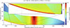 |
Figure 5. Distribution of particle positions for test case 2c (note the a logarithmic scale!). One can clearly recognize the downward- and upward refraction in the downwind- and upwind domain, respectively. Along the boundary of the shadow zone in the upwind domain a significantly increased number of particle positions can be observed. (a) Case 2c, wind speed u r (10 m)=5.0 m/s. |
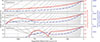 |
Figure 6. Results for test case 2, computed using Akumet with a grid width of 8 m for a frequency of 100 Hz. Sound pressure level is given in red, sound rays are shown in grey, and the number of particles per grid cell in blue. |
Figure 5 shows – for test cases 2c – the distribution of the particle positions within the computational domain including a zoom on the region in which the sound pressure level increase occurs. One can clearly see the expected downward-refraction in the downwind domain as well as the upward-refraction in the upwind domain, eventually leading to the formation of a shadow zone. However, one can also observe a significant accumulation of particle positions along the boundary of the shadow zone as well as an “overlap” of refracted and non-refracted particle positions above the shadow zone. Generally, the effect is more pronounced in case with a wind speed of 5.0 m/s at 10 m of height compared to the case with a lower wind speed of 2.5 m/s. Note that the number of particle positions is shown on a logarithmic scale.
While Figure 5 shows all particle positions within the computational domain, Figure 6 highlights the total number of particle positions per control volume within the ground layer (i.e., z ∈ [0, 8]). As mentioned in Section 2, a control volume is a volume (3D) or area (2D) of a given size in which the particle positions are counted and evaluated to receive the final sound pressure level. These numbers of particles per control volume within the ground layer are shown by the blue dash-dotted curve, the sound pressure level is shown by the red solid line and selected sound rays are indicated in grey.
Compared to test case 1, the adjustments and simplifications made for test case 2 lead to an enhanced effect of increased sound pressure level in the upwind domain. In case of a wind speed of 5 m/s, this increase was preceded by an accentuated decrease in sound pressure level, which could not be observed to this extent in test case 1. For the reduced wind speed of 2.5 m/s the drop in sound pressure level is significantly lower and occurs further away from the source. The area of increased sound pressure level however stretches out much further and, as well as the drop, occurs at a greater distance from the source. Finally, as can be expected, the sound pressure level in calm conditions decreases monotonously without any rises or drops.
Looking more closely at the sound rays, one finds that the drops in sound pressure level occur in the areas where the first sound rays, those still moving downwards and those that have already been refracted upwards, are intersecting. This is often interpreted as a caustic in ray tracing models, since the cross-sectional area of the ray tube approaches zero. In the particle-based approach, however, this phenomenon is understood as follows: A higher number of particles in that area is visible, and, depending on the frequency and phase shift, this leads to destructive interference (resulting in the sound pressure level to drop, red curve). Further upwind, the number of particles decreases again, but so do the effects of interference, leading to a relative increase in sound pressure level. The number of particles is, due to the additional upwards refracted sound rays in that area, still higher than it was before the drop, and therefore is the sound pressure level.
Finally, the maximum in sound pressure level (around x = −700 m in Fig. 6, bottom) is caused by the increased number of sound particles. As the sound energy emitted by the source is distributed among the sound particles, areas with an increased number of particles directly translate to areas of increased sound energy.
4.2 Test case 3 – Analysis of different refractive conditions
Section 4.1 showed how the intersection of refracted and non-refracted sound rays causes an increase in available sound energy and the respective sound pressure level in the upwind domain. This requires conditions in which the refractive coefficient decreases with height (non-linear sound propagation profile). Accordingly, in case of a height-invariant refractive coefficient, i.e., a linear vertical gradient of the effective sound speed, no intersection of sound-rays (wave-fronts) can occur. Therefore, no increase in sound pressure level in the upwind domain should be observable, and the sound pressure level near the ground must be lower in upwind- than in downwind conditions. Furthermore, we can construct a logarithmic temperature profile T(z) in Kelvin with:
 (15)
(15)
where T ground is the temperature at the ground, given in Kelvin, and T r describes the reference temperature at 10 m above ground in Celsius. This leads to a sound propagation that, within each height level, is point-symmetric around the source and shows the same characteristic behaviour as in case of a logarithmic wind profile in direct upwind direction. In order to verify these hypotheses, test case 3 was set up, using a total of four atmospheric profiles, where a homogeneous atmosphere is used as a reference.
The simulation results of test case 3 are shown in Figures 7 and 8. The respective configurations are summarized in Table 4 (basic setup) and Table 5 (specific profiles). The computational domain remained the same as in test case 1. A distinction is made between the following situations:
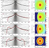 |
Figure 7. Results of Akumet (test cases 3a–3d, see Tabs. 4 and 5): Left side: vertical cross-sections through y = 0, indicating the sound rays resulting from the particle motion (grey, left axis). The sound pressure level through the source position is given in red (right axis). Right side: according sound pressure level fields at 4 m above ground are shown. |
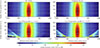 |
Figure 8. Results of Akumet (test cases 3a–3d, see Tabs. 4 and 5): Vertical cross section of the sound pressure level field for 100 Hz point source with source height 75 m and absorbing ground for different atmospheric conditions. |
Basic setup for case 3.
Atmospheric profiles for case 3.
Homogeneous sound propagation conditions: sound particles move along straight paths and therefore sound propagates equally in all directions.
Linear wind profile: upwind travelling sound particles move on convex paths (upward refraction), downwind travelling sound particles move on concave paths (downward refraction), no intersection of resulting sound rays and no increase in sound pressure level within the upwind domain. Formation of a shadow zone at –600 m.
Logarithmic wind profile: sound particles travelling in upwind direction move on convex paths (upward refraction), downwind travelling sound particles move on concave paths (downward refraction), intersection of resulting sound rays starting at –450 m, accompanied by a significant increase in sound pressure level within the upwind domain. Formation of a shadow zone at –800 m.
Logarithmic temperature profile: both, upwind and downwind travelling sound particles move on convex paths (upward refraction), leading to intersection of resulting sound rays starting at –450 m, accompanied by a significant increase in sound pressure level within the upwind and downwind domain. Formation of a shadow zone at –800 m. The sound propagation is symmetric around the source as the sound propagation conditions are symmetric around the source as well.
5 Comparison with Aku3d
This model approach was set up in order to verify that increased sound levels in the upwind domain can also be observed within a different model. Here, a full-wave model like Aku3d is particularly well suited as it directly solves the wave-propagation and all physical effects. As mentioned in Section 2Aku3d could simulate a Gaussian pulse pressure as initial conditions or a point source with distinct frequency.
This section was designed to be comparable to test case 1 and case 3. Due to the increased computational cost of the full-wave model, only 2-dimensional simulations have been performed, where the domain size is given by
![Mathematical equation: $$ \begin{aligned}&x : [-1600, 1600] \, \mathrm{m}, \\&z : [0, 900]\,\mathrm{m}. \end{aligned} $$](/articles/aacus/full_html/2026/01/aacus250062/aacus250062-eq33.gif)
The width of the domain is larger compared to test case 1 in order to catch the beginning of the shadow zone. The height of the domain has been chosen in order to avoid the influence of spurious reflections from the upper boundary back into the actual domain of interest (lowest 100 m).
Perfectly absorbing ground conditions are applied since, all interference patterns shown later are solely a result of refraction. First, the source is defined as a Gaussian pulse with FWHM = 2 m, or σ ≈ 0.85, respectively (see (10) and (11)). Therefore, the highest relevant frequency f is around 80 Hz. Due to the Gaussian shape of the pulse also higher frequencies still exist and slightly impact the result. In Aku3d, each wave has to be resolved with at least 6–8 grid cells. The maximum wind speed within the domain can be computed using (14) where u (900 m)≈11.8 m/s. The sound speed is defined as 340.0 m/s, such that the lowest effective wind speed – resulting in the shortest possible wave-length – is min(ceff)=328.2 m/s. For a frequency of 20 Hz this gives a minimum wave-length of
Resolving this wave-length with 8 grid cells would therefore result in a grid width of about 0.5 m. In order to also account for frequencies exceeding 80 Hz, the grid width was further reduced by a factor of 2, resulting in a final grid width of 0.25 m. The time step was calculated via the CFL-criterion, using a CFL-number of 0.5. Taking into account the grid width and the maximum effective sound speed, max(ceff)=351.8 m/s results in a time step of △t = 0.00035 s. The meteorological conditions are equal to those used for the Akumet simulations. The general setup of the Aku3d simulations are summarized in Table 6.
Basic setup for case 4.
5.1 Comparison to Case 1
Figure 9 shows the sound energy density level field up to 600 m above ground. The upwind domain shows a significant increase in sound level in ground proximity that is comparable to the effects found in the Akumet test cases 1. Just as well, the area of increased sound level “detaches” from the ground with increasing longitudinal distance from the source, where the shadow zone starts to form right below this area of increased sound level. In comparison to the Akumet test cases, the shadow zone is less pronounced.
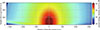 |
Figure 9. Results of Aku3d simulation (case 4, see Tab. 6) for Gaussian pulse with source height of 75 m and logarithmic wind profile, wind direction from left to right. |
A more detailed look at the sound levels is given in Figure 10. Figure 10a shows the sound energy density levels at 4 selected heights. At a distance of ∼500 m upwind of the source, the increase of sound level becomes apparent at the 3 lower height levels (4 m, 12 m and 20 m). At source height, this increase starts to be noticeable at a larger distance from the source. Figure 10b shows the differences between the upwind- and the downwind-domain, i.e., positive sound level differences indicate that the sound levels in the upwind domain are exceeding those downwind of the source. Here it becomes evident that the sound levels in the upwind domain actually exceed the downwind levels all the way from the source to the beginning of the formation of a shadow zone in the upwind domain. At ground level the maximum in difference is reached around 750 m upwind of the source, where the sound levels exceed the downwind ones by about 4 dB. However, the differences remain larger than 1 dB (hearing threshold) up to a distance of ∼1250 m upwind of the source.
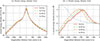 |
Figure 10. Results of Aku3d simulation (case 4, see Tab. 6): Sound energy density levels simulated using Aku3d as well as the respective differences between upwind and downwind. (a) Sound energy density level. (b) △ Sound energy density level. |
Since the source is defined as a Gaussian pulse, it is not restricted to a single grid cell (as in test case 1a), but stretches out over multiple cells with a FWHM of 2 m. This corresponds to a FWHM of the frequency distribution of ∼150 Hz. So, higher as well as much lower frequencies are included in this initial pulse. The low frequency contents and the broadband characteristic of the source dominate and blur the result. Therefore, the findings from case 4 resemble those of test case 1b (see Fig. 4b) more than those of test case 1a (see Fig. 4a). Test cases 1b and 4 both show an increase in upwind sound pressure level of about 4 dB compared to the downwind domain, as well as a delayed onset of the shadow zone compared to test case 1a.
5.2 Comparison to Case 3
The FDTD model, simulating either a Gaussian source or a point source with a distinct frequency of 100 Hz, allows for the demonstration of caustic formation when waves of various or single wavelengths interfere, respectively. The distinct single frequency helps to highlight the caustic effect that looks smaller when the broadband source is used. Additionally, a comparison with different meteorological conditions are provided for the two source types. This allows to compare the Akumet results achieved in Section 4.2 which demonstrated the sensitivity upon the meteorological fields. These test cases examine whether the upwind level rise predicted by the particle model (Akumet) can also be reproduced with the full-wave solver.
First, the source placed at (0, 75) m is defined as a Gaussian pulse with FWHM = 10 m representing very low frequencies. The basic parameters of the setup of Aku3d remain according to Table 6 and additionally for the six atmospheric profiles the parameters shown in Table 7 are applied. Then, the same meteorological conditions were applied for a monochromatic point source at 100 Hz.
Atmospheric profiles for case 4 (a to f).
Contour plots of vertical cross sections of all simulation result allow a broad comparison of both model approaches. The base line simulation with a homogeneous atmosphere, the constant gradient wind as well as the rising wind speed thus higher shear near the ground and the symmetric temperature profile was studied with both models. Figure 11 shows the contour fields for the Gaussian pulse for the different meteorological conditions. Here, the sound pressure level increase in the upwind domain is less visible than for other frequency ranges. Nevertheless, it can be seen, that in both models e.g., the nonlinear temperature field profile reproduces the symmetric structure as found in Akumet, see Figure 8.
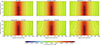 |
Figure 11. Results of Aku3d simulations (test cases 4a–4f, see Tabs. 6 and 7): Sound–pressure contours for a broadband Gaussian pulse (FWHM ≈ 10 m, source height 75 m) over a totally absorbing ground. Six atmospheric scenarios are shown: calm, constant shear, logarithmic winds with U10 = 2.5, 5.0 and 10.0 m/s, and a logarithmic temperature inversion. |
Figure 12 shows the contour fields for the 100 Hz point source. Here an interference structure is well visible not based on reflection, but on refraction. For this single frequency case interference patterns are visible even better than in Akumet. In the particle-based model the evaluation resolution is not sufficient to visualize this effect. Furthermore, the same sound pressure level increase in the upwind domain as for the Gaussian pulse source is visible, especially in the panel with U10 = 5 m/s and U10 = 10 m/s. Both source types display the upwind enhancement zone and the emerging shadow boundary. Comparing Figures 11 and 12 confirms that, for the Gaussian pulse, the sound pressure level variations under different atmospheric conditions are less pronounced than the case of the 100 Hz point source.
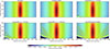 |
Figure 12. Results of Aku3d simulations (test cases 4a–4f, see Tabs. 6 and 7): Sound–pressure contours for a monochromatic point source at 100 Hz (same geometry as Fig. 11). The coherent tone reveals the interference stripes in the upwind lobe. |
To assess the results quantitatively the following line plots show, that for the Gaussian pulse (Fig. 13) the sound pressure level increase in upwind direction doesn’t exceed 0.7 dB but follows a clear trend: weak shear, orange line, (U10 = 2.5 m/s) peaks at about 0.40 dB, moderate shear, green line, (U10 = 5 m/s) at roughly 0.55 dB, and strong shear, red line, (U10 = 10 m/s) at 0.65 dB; the logarithmic temperature profile (purple line) behaves like the strong-shear case and attains approximately 0.70 dB. The place of the maximal sound pressure level increase changes with growing shear from x = −1000 m to x = −500 m.
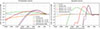 |
Figure 13. Upwind level excess (Δ-SPL) at 4 m above ground for the Gaussian-pulse case and for the 100 Hz point source, referenced to the calm baseline. |
With the 100 Hz point source (Fig. 13), the effect is much larger. The increase reaches about 4.5 dB under weak shear (orange line), 6 dB under moderate shear (green line), and 6–7 dB under strong shear(red line) or the logarithmic temperature profile (purple line), with the respective maxima lying between x = −800 m and x = −400 m. The shadow zone for the moderate shear, green line, U10 = 5 m/s) begins at x = −780 m very similar to the results obtained from Akumet, see Figure 7. Although the coherent tone exhibits fine interference fringes, its overall behavior mirrors that of the broadband case, indicating that energy focusing, rather than phase locking, governs the gain.
For both source configurations, the Aku3d results reproduce the same upwind rise and fall pattern seen in Akumet even though their peak magnitudes differ, confirming that a non-linear vertical gradient in effective sound speed, arising from wind shear or temperature that drives the focusing mechanism. Figures 11–13 confirm the upwind sound pressure level increases for every non-linear profile and show how its magnitude depends on shear strength.
6 Summary
This study investigated the phenomenon of increased sound pressure levels in the upwind domain of elevated sound sources, such as wind turbines, caused by upward refraction. Our primary objective was to explain the physical origin of potential upwind sound pressure level (SPL) increases associated with caustics, an aspect often neglected in literature. We demonstrate that upwind SPL increases can occur under specific atmospheric conditions, particularly with a logarithmic wind profile, resulting from the combination of sound focusing due to refraction and interference effects. This leads to a characteristic interference pattern where SPL can increase.
We analysed this effect using two distinct modelling approaches: The FDTD model (Aku3d) and a geometrical-based particle model (Akumet). Both models show qualitatively consistent results, yet quantitative assessment remains challenging due to specific model inherent limitations. For example, for Aku3d, accurately representing a totally absorbing ground at low frequencies can be challenging, and it incurs high computational costs for high frequencies. Akumet, while suitable for high frequencies and long-range propagation, has limitations in resolving interference patterns finely due to its predefined cell size requirement for particle counting. Nevertheless, both models consistently show the positions and spatial extent of sound focusing and interference in the upwind domain, with only absolute SPL amplitudes differing based on model restrictions.
Contrary to the common expectation that, due to upward refraction and sound shadow formation, sound levels are always lower in the upwind region, simulation results from both models reveal that sound levels in the upwind domain can exceed those in the downwind domain under certain conditions. For instance, if the vertical gradient of the effective sound speed decreases logarithmically with increasing height. This superposition leads to an increase in available sound energy near the ground. Depending on the vertical gradient of ceff, the effect can range from mild but widespread to strong but locally limited.
Through various test cases, this study elucidated the effect, demonstrating upwind sound pressure level increases of several dB relative to downwind conditions. The particle model (Akumet) predicted an increase of up to 10 dB, which should be considered as an upper limit due to inherent limitations that can lead to an overestimation. In contrast, our wave-based model (Aku3d) provides a more reliable reference, predicting a maximum increase of 6.5 dB, which better reflects the physical phenomena and our observations.
Test case 1 examined the effects of different sound source configurations, comparing single point sources vs. multiple point sources, on sound propagation under logarithmic wind profiles and for a whole frequency spectrum. The results showed that the sound level in the upwind region for a single source is characterized by a sharper increase compared to a multi-point source, suggesting that in measurements, this effect might be less obvious to be detected. By restricting the domain to 2D, disabling additional effects like ground reflections and using a single frequency, the origin of the increased sound level in the upwind region could be isolated. The results also showed that the effect is more pronounced at higher wind speeds and is caused by focusing of sound energy (sound particles) due to refraction effects. Test case 3 investigated the influence of different refractive conditions on sound propagation using four different atmospheric profiles: homogeneous, linear wind, logarithmic temperature, and logarithmic wind. The results showed that the effect only occurs under logarithmic profiles, confirming that it is related to the curvature and intersection of sound rays. Finally, the results obtained using the particle-based model (Akumet) were compared to those of the wave-based model (Aku3d) in test cases 4a–4f with two different source representations (point source and Gaussian distributed source. We repeated the meteorological conditions used in Akumet and compared the results of both models, which showed that both models predict an increase in sound level in the upwind region, suggesting that the effect is not limited to a specific model.
The findings of this study suggest that the possibility of increased sound levels in the upwind domain has to be considered when assessing the sound propagation from elevated sources, particularly under conditions with non-linear (e.g., logarithmic) wind and temperature profiles. The results also emphasize the importance of using accurate meteorological data and sound propagation models for evaluating the environmental impact of sound sources.
7 Conclusion
The predicted sound level increase represents a maximum value under specific, idealized circumstances, such as a point source in an environment with a perfectly smooth logarithmic wind profile, no turbulence or ground reflections. We acknowledge that the complexity of real-world conditions makes this specific effect challenging to isolate and measure, which is why it has not been widely documented. Nevertheless, complaints from local residents about uncommonly high sound levels in the upwind region of sources like wind turbines suggest this phenomenon may be relevant in practice. This work, therefore, may serve to highlight the potential for significant sound level increases in upwind propagation with elevated sources, encouraging further scientific investigation into this complex phenomenon.
Acknowledgments
The authors extend their sincere gratitude to the two anonymous reviewers for their thoughtful comments and constructive suggestions, which significantly strengthened this manuscript.
Conflicts of interest
The authors declare that they have no conflicts of interest. The authors declare that they have no known competing financial interests or personal relationships that could have appeared to influence the work reported in this paper.
Data availability statement
The data that support the findings of this study are available from the corresponding author upon reasonable request.
References
- T.F.W. Embleton: Tutorial on sound propagation outdoors. The Journal of the Acoustical Society of America 100, 1 (1996) 31–48. [Google Scholar]
- E.M. Salomons: Computational Atmospheric Acoustics. Kluwer Academic Publishers, Dordrecht, The Netherlands, 2001. [Google Scholar]
- K. Attenborough: Review of ground effects on outdoor sound propagation. The Journal of the Acoustical Society of America 86, 4 (1988) 1493–1532. [Google Scholar]
- International Organization for Standardization: Acoustics – attenuation of sound during propagation outdoors – part 2: general method of calculation. Technical Report ISO 9613-2:1996, International Organization for Standardization, Geneva, Switzerland, 1996. [Google Scholar]
- G.A. Daigle: Effects of atmospheric turbulence on the intermittent amplification of sound propagating along a ground surface. The Journal of the Acoustical Society of America 73, 2 (1983) 669–675. [Google Scholar]
- J.E. Piercy, T.F.W. Embleton, L.C. Sutherland: Review of noise propagation in the atmosphere. The Journal of the Acoustical Society of America 61, 6 (1977) 1403–1418. [Google Scholar]
- B. Cotté: Coupling of an aeroacoustic model and a parabolic equation code for long range wind turbine noise propagation. Journal of Sound and Vibration 422 (2018) 343–357. [CrossRef] [Google Scholar]
- J. Colas, A. Emmanuelli, D. Dragna, P. Blanc-Benon, B. Cotté, R.J.A.M. Stevens: Impact of a two-dimensional steep hill on wind turbine noise propagation. Wind Energy Science, 9 (2024) 1869–1884. [Google Scholar]
- D. Luquet, R. Marchiano, F. Coulouvrat: Long range numerical simulation of acoustical shock waves in a 3d moving heterogeneous and absorbing medium. Journal of Computational Physics 379 (2019) 237–261. [CrossRef] [Google Scholar]
- H.H. Brouwer: A ray acoustics model for the propagation of aircraft noise through the atmosphere. International Journal of Aeroacoustics 5, 6 (2014) 363–384. [Google Scholar]
- D. Heimann: Modelling sound propagation from a wind turbine under various atmospheric conditions. Meteorologische Zeitschrift 27, 4 (2018) 265–275. [Google Scholar]
- C.D. Doolan, D.J. Moreau, L.A. Brooks: Wind turbine noise mechanisms and some concepts for its control. Acoustics Australia 40, 1 (2012) 7–13. [Google Scholar]
- V.E. Ostashev, D.K. Wilson: Acoustics in Moving Inhomogeneous Media, 2nd edn. CRC Press, Boca Raton, FL, 2015. [Google Scholar]
- K. Elsen, F. Bertagnolio, A. Schady: Sound-propagation in wind energy: a code2code-comparison, in: 10th Convention of the European Acoustics Association, 2023, pp. 3821–3838. [Google Scholar]
- D. Heimann, G. Gross: Coupled simulation of meteorological parameters and sound level in a narrow valley. Applied Acoustics 56 (1999) 73–100. [Google Scholar]
- A.D. Pierce: Acoustics: An Introduction to Its Physical Principles and Applications. McGraw-Hill, New York, 1981. [Google Scholar]
- R. Blumrich, F. Coulouvrat, D. Heimann: Variability of focused sonic booms from accelerating supersonic aircraft in consideration of meteorological effects. The Journal of the Acoustical Society of America, 118:696, 2005. [Google Scholar]
- D. Heimann, Y. Käsler, G. Gross: The wake of a wind turbine and its influence on sound propagation. MetZet 20, 4 (2011) 449–460. [Google Scholar]
- M. Kästner, D. Heimann: Effect of atmospheric variability and aircraft flight parameters on the refraction of sonic booms. Acta Acustica 96 (2010) 425–436. [Google Scholar]
- S. Gharbi, A. Schady: Investigation of Ground Effects and Atmospheric Conditions on Noise Perception from Small Aircraft Technologie. Quiet Drones Conference 2024, Manchester, UK, 2024. [Google Scholar]
- A. Feldhusen-Hoffmann, L. Bertsch, M. Pott-Pollenske, V. Domogalla, M. Kreienfeld, N. Dörge: Noise and local pollutants of small aircraft: overview of simulation activities and of the first flight test within the DLR project L2INK. San Diego, AIAA AVIATION 2023 Forum, 2023. [Google Scholar]
- R. Blumrich, D. Heimann: A linearized eulerian sound propagation model for studies of complex meteorological effects. JASA 112, 2 (2002) 446–455. [Google Scholar]
- D. Heimann, R. Karle: a. JASA 119, 6 (2006) 3813–3821. [Google Scholar]
- J.-P. Berenger: A perfectly matched layer for the absorption of electromagnetic waves. Journal of Computational Physics, 114, 2 (1994) 185–200. [Google Scholar]
- K. Heutschi, M. Horvath, J. Hofmann: Simulation of ground impedance in finite difference time domain calculations of outdoor sound propagation. Acta Acustica United with Acustica 91, 1 (2005) 35–40. [Google Scholar]
- D. Dragna, B. Cotté, P. Blanc-Benon, F. Poisson: Time-domain simulations of outdoor sound propagation with suitable impedance boundary conditions. AIAA Journal 49, 7 (2011) 1420–1428. [Google Scholar]
- M.E. Delany and E.N. Bazley: Acoustical properties of fibrous absorbent materials. Applied Acoustics 3 (1970) 105–116. [Google Scholar]
- Y. Miki: Acoustical properties of porous materials – modifications of Delany–Bazley models. The Journal of the Acoustical Society of America 11, 1 (1990) 19–24. [Google Scholar]
- D. Heimann, A. Englberger, A. Schady: Sound propagation through the wake flow of a hilltop wind turbine – a numerical study. Wind Energy 21, 8 (2018) 650–662. [Google Scholar]
- D. WindGuard: Schallemissionsmessungen an einer Windenergieanlage – Bericht MN15016.A1. Technical report, Deutsche WindGuard, 2015. [Google Scholar]
- International Organization for Standardization: Acoustics – acoustics; attenuation of sound during propagation outdoors; part 1: calculation of the absorption of sound by the atmosphere. Technical Report ISO 9613-1:1996, International Organization for Standardization, Geneva, Switzerland, 1996. [Google Scholar]
Cite this article as: Baumann K. Gharbi S. Juliust H. & Schady A. 2025. How elevated sources can cause local increases of sound pressure levels in the upwind domain. Acta Acustica, 10, 5. https://doi.org/10.1051/aacus/2025071.
All Tables
All Figures
|
Figure 1. Simulated sound pressure level at ground level (4 m above ground) for test case 1. The increased sound levels in the upwind domain are clearly visible for both source setups, but more pronounced for the single point source setup (a). (a) Case 1a: Sound source representation using a single point source at the nacelle. (b) Case 1b: Sound source representation using 36 point sources, distributed along the rotational plane. |
| In the text | |
|
Figure 2. Vertical cross section of the sound pressure level field through the wind turbine (y = 0), shown for the lowest 80 m. The 4 black dashed lines indicate the mean heights of the sound pressure level curves shown in Figure 3. (a) Case 1a (single source). (b) Case 1b (multi-source). |
| In the text | |
|
Figure 3. Sound pressure levels through y = 0 for selected heights (4 m, 12 m, 20 m and 76 m) above ground as indicated by the black dotted lines in Figure 2. (a) Case 1a. (b) Case 1b. |
| In the text | |
|
Figure 4. Differences in sound pressure levels between upwind and downwind, through y = 0 for selected heights (4 m, 12 m, 20 m and 100 m) above ground as indicated by the black dotted lines in Figure 2. (a) Case 1a. (b) Case 1b. |
| In the text | |
|
Figure 5. Distribution of particle positions for test case 2c (note the a logarithmic scale!). One can clearly recognize the downward- and upward refraction in the downwind- and upwind domain, respectively. Along the boundary of the shadow zone in the upwind domain a significantly increased number of particle positions can be observed. (a) Case 2c, wind speed u r (10 m)=5.0 m/s. |
| In the text | |
|
Figure 6. Results for test case 2, computed using Akumet with a grid width of 8 m for a frequency of 100 Hz. Sound pressure level is given in red, sound rays are shown in grey, and the number of particles per grid cell in blue. |
| In the text | |
|
Figure 7. Results of Akumet (test cases 3a–3d, see Tabs. 4 and 5): Left side: vertical cross-sections through y = 0, indicating the sound rays resulting from the particle motion (grey, left axis). The sound pressure level through the source position is given in red (right axis). Right side: according sound pressure level fields at 4 m above ground are shown. |
| In the text | |
|
Figure 8. Results of Akumet (test cases 3a–3d, see Tabs. 4 and 5): Vertical cross section of the sound pressure level field for 100 Hz point source with source height 75 m and absorbing ground for different atmospheric conditions. |
| In the text | |
|
Figure 9. Results of Aku3d simulation (case 4, see Tab. 6) for Gaussian pulse with source height of 75 m and logarithmic wind profile, wind direction from left to right. |
| In the text | |
|
Figure 10. Results of Aku3d simulation (case 4, see Tab. 6): Sound energy density levels simulated using Aku3d as well as the respective differences between upwind and downwind. (a) Sound energy density level. (b) △ Sound energy density level. |
| In the text | |
|
Figure 11. Results of Aku3d simulations (test cases 4a–4f, see Tabs. 6 and 7): Sound–pressure contours for a broadband Gaussian pulse (FWHM ≈ 10 m, source height 75 m) over a totally absorbing ground. Six atmospheric scenarios are shown: calm, constant shear, logarithmic winds with U10 = 2.5, 5.0 and 10.0 m/s, and a logarithmic temperature inversion. |
| In the text | |
|
Figure 12. Results of Aku3d simulations (test cases 4a–4f, see Tabs. 6 and 7): Sound–pressure contours for a monochromatic point source at 100 Hz (same geometry as Fig. 11). The coherent tone reveals the interference stripes in the upwind lobe. |
| In the text | |
|
Figure 13. Upwind level excess (Δ-SPL) at 4 m above ground for the Gaussian-pulse case and for the 100 Hz point source, referenced to the calm baseline. |
| In the text | |
Current usage metrics show cumulative count of Article Views (full-text article views including HTML views, PDF and ePub downloads, according to the available data) and Abstracts Views on Vision4Press platform.
Data correspond to usage on the plateform after 2015. The current usage metrics is available 48-96 hours after online publication and is updated daily on week days.
Initial download of the metrics may take a while.