| Issue |
Acta Acust.
Volume 9, 2025
|
|
|---|---|---|
| Article Number | 15 | |
| Number of page(s) | 12 | |
| Section | Ultrasonics | |
| DOI | https://doi.org/10.1051/aacus/2025002 | |
| Published online | 20 February 2025 | |
Scientific Article
Ultrasonic wave field image augmentation in PZT sensors using generative machine learning and Coulomb coupling
1
Department of Mathematics, Indian Institute of Technology Guwahati, Assam, 781039, India
2
Department of Civil Engineering, Indian Institute of Technology Guwahati, Assam, 781039, India
3
Department of Physics and Technology, UiT The Arctic University of Norway, Tromsø, Norway
* Corresponding author: This email address is being protected from spambots. You need JavaScript enabled to view it.
Received:
23
September
2024
Accepted:
9
January
2025
Abstract
This paper presents an approach to overcome the time-intensive nature of the Coulomb coupling imaging method by employing Generative Adversarial Networks (GANs) for data augmentation. Coulomb coupling, an experimental technique, is essential for visualizing ultrasonic wave propagation in piezoelectric materials and is valuable in various domains including materials research. It provides valuable insights such as finding mechanical properties and detecting anomalies in piezoelectric materials. However, the efficiency of this method is hindered by traditional time expansive point-by-point scanning. Integrating advanced machine learning into Coulomb coupling imaging has emerged as a promising solution to address this issue. Nonetheless, the lack of sufficient data has been a significant challenge. The key contribution is the use of GANs to create synthetic yet realistic images from a limited set of real data, effectively overcoming the issue of data scarcity. A large number of artificial images were successfully generated, expediting model training and enhancing generalization. This study is the first to use GANs in Coulomb coupling imaging, showing its transformative potential. By overcoming data limitations, the proposed approach enhances Coulomb coupling imaging and enables its integration with advanced technologies like AI-driven predictive modeling and real-time adaptive imaging. This opens new frontiers for applications in materials science and other imaging modalities.
Key words: Coulomb coupling / Piezoelectric ceramics / Acoustic imaging / Generative adversarial networks
© The Author(s), Published by EDP Sciences, 2025
 This is an Open Access article distributed under the terms of the Creative Commons Attribution License (https://creativecommons.org/licenses/by/4.0), which permits unrestricted use, distribution, and reproduction in any medium, provided the original work is properly cited.
1 Introduction
Coulomb coupling imaging has become a valuable technique in materials research, offering significant insights into the mechanical properties of materials and enabling the detection of anomalies in piezoelectric materials [1, 2]. Coulomb coupling in piezoelectric materials refers to the phenomenon where electrical energy is converted into acoustic energy through the interaction between the electric field gradient and the strain gradient. At high voltage, the electric field concentrates at the point contact tip of the Coulomb probes. In the Coulomb coupling process, this localized electric field at the probe’s point contact interacts with the material’s mechanical properties through a strain gradient. The localized strain gradient at the point contact excites phonons in the piezoelectric material, leading to the generation and propagation of ultrasonic waves within the samples. Surface discontinuities in geometrical and material properties result in a highly localized electric field, functioning as a secondary or passive wave source. The frequency-dependent behavior of the piezoelectric transducer arises from the resonance and geometrical interference associated with the piezo coupling. Applying an electric field to a piezoelectric material induces mechanical vibrations, or phonons, through the piezoelectric effect. These phonons propagate through the crystal lattice, transmitting energy as ultrasonic waves and enabling various applications in sensing, actuation, and wave generation [3]. Detection methods based on the same piezoelectric principles convert these mechanical vibrations back into electrical signals, enabling detailed analysis of phonon behavior. This approach provides crucial insights into material characteristics such as elasticity, crystal defects, and thermal properties, making it an invaluable tool in material science [4, 5]. High-resolution images provide a noninvasive method for micro-structural characterization, allowing researchers to explore both surface and subsurface mechanical properties in detail. This technique enables the monitoring of the structural health of piezoelectric materials, the examination of surface and subsurface defects, and the study of anisotropic phonon propagation [5, 6]. These capabilities are crucial for understanding material behavior and ensuring the reliability and performance of piezoelectric components.
Coulomb coupling imaging offers detailed insights and broad applications but is limited by the slow, time-intensive point-by-point scanning method. This approach hampers high-throughput and real-time analysis, emphasizing the need for faster, more efficient imaging techniques to unlock its full potential. Each point on the sample must be individually scanned, which involves precise positioning and data acquisition, resulting in a slow overall process. This challenge becomes even more pronounced when dealing with small samples, where the need for high-resolution imaging requires finer steps and more data points, significantly increasing the scanning time. The laborious and time-consuming nature of the point-by-point scanning approach presents a substantial hurdle, limiting the efficiency and practicality of Coulomb coupling imaging in research and industrial applications. Extended scanning times can lead to potential issues such as sample drift, thermal fluctuations, and increased wear on the scanning equipment, which can further affect the accuracy and reliability of the results. Thus, while Coulomb coupling imaging offers a wealth of valuable information regarding mechanical properties, structural health, and defect detection in piezoelectric materials, the significant time required for thorough scans, particularly for minute samples, poses a considerable challenge. Addressing this issue is crucial to enhance the technique’s overall utility and applicability.
In recent years, a promising avenue for enhancing the efficiency of Coulomb coupling imaging has emerged through the integration of machine learning techniques [1, 7–9]. However, the successful implementation of these techniques relies heavily on the availability of extensive datasets, which are often scarce in the field of Coulomb coupling imaging. To overcome this limitation, this work introduces a data augmentation technique based on Generative Adversarial Networks (GANs) [10]. Data augmentation plays a vital role in machine learning, particularly in scenarios where the availability of real-world data is limited. By generating synthetic but realistic-looking data, data augmentation expands the diversity and size of training datasets, leading to more robust and accurate models. Among the various techniques used for data augmentation, GANs have emerged as a powerful tool. GANs are a class of artificial intelligence algorithms that learn the underlying patterns of a given dataset and use this knowledge to generate high-quality synthetic data.
This paper introduces the application of GANs to the field of Coulomb coupling imaging, demonstrating the feasibility of generating a substantial number of synthetic, realistic images from a limited set of real images. This approach allows us to overcome the challenge of data scarcity in Coulomb coupling imaging, enabling the generation of a more extensive dataset for training machine learning models. By employing GANs, we have successfully produced a significant number of fake images that closely mimic the characteristics of real Coulomb coupling images. This augmentation not only accelerates the training process but also enhances the robustness and generalization capabilities of machine learning models applied to Coulomb coupling. By incorporating diverse and augmented data into the training sets, the models become more proficient at recognizing patterns and anomalies in various conditions, leading to more accurate and reliable predictions. This improvement in model performance is crucial for advancing the application of machine learning in the detailed analysis of mechanical properties and defects within piezoelectric materials, ultimately contributing to more efficient and effective research and industrial processes.
To the best of our knowledge, this study represents the first exploration of GANs in the context of Coulomb coupling data augmentation. The novelty of this work lies in the application of artificial intelligence techniques to tackle the fundamental challenge of improving Coulomb coupling imaging. This challenge involves addressing the limitations in image acquisition processes, which are often time-consuming and constrained by the availability of comprehensive data. By leveraging AI, the proposed approach enhances data interpretation and optimizes the imaging workflow, thereby overcoming these barriers and contributing to the advancement of Coulomb coupling imaging capabilities. The subsequent sections of this paper will delve into the methodology, results, and implications of the data augmentation technique, shedding light on the potential it holds for the broader field of Coulomb coupling (Fig. 1).
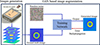 |
Figure 1 This figure depicts the overall strategy used in this paper. First, real data (ground truth) is acquired. This is followed by GAN-based data augmentation. Real images and random noise input images are fed into the network used to train. The network output is further used as error back-propagation to train the network. |
2 Relation to prior work
The augmentation of existing datasets through transforming original data is pivotal for enhancing the diversity and richness of training datasets. This encompasses a spectrum of image manipulation techniques, ranging from fundamental affine transformations to intricate distortions [11].
2.1 Transformation of original data
The augmentation of existing datasets through the transformation of original data is crucial for enhancing the diversity and richness of training datasets [12]. This category includes a wide range of image manipulation techniques, from basic affine transformations to more complex distortions. Affine transformations, a subset of geometrical transformations, preserve the geometric properties of lines and parallelism, although they do not necessarily maintain distances and angles. Operations such as translation, rotation, flipping, scaling, cropping, and shearing maintain the aspect ratio of images along one or more axes of symmetry. These transformations are fundamental in ensuring that neural networks can recognize objects regardless of their orientation or position in the image. Erasing transformations involve selecting a defined region within an image and replacing the chosen pixels with either a fixed intensity value or random noise. Initially developed for the RGB domain, this technique increases robustness to occlusions, preventing neural networks from relying solely on simple detection patterns and reducing spurious correlations due to dataset biases. Pixel-level transformations modify pixel values in a detailed manner, affecting image characteristics such as brightness, contrast, saturation, and noise. These modifications are essential for enhancing the resilience of deep neural networks (DNNs) across different scanners and imaging protocols. By addressing potential variations in pixel distribution, these transformations ensure that DNNs remain robust and effective despite differences in imaging conditions and equipment. This adaptability is crucial for deploying machine learning models in diverse real-world scenarios, where imaging conditions can vary significantly [13, 14].
2.2 Generation of artificial data
Transformation-based techniques enrich datasets, but generating artificial or synthetic samples introduces greater diversity and complexity, surpassing traditional methods. This can be achieved through feature mixing or ad-hoc modeling strategies tailored to specific imaging tasks. Feature mixing methods, such as the mix-up technique, combine samples from the original dataset to create new synthetic samples, enhancing the generalization capabilities and robustness of neural networks [15]. The mix-up technique involves creating new training samples by linearly combining pairs of examples and their labels. This approach encourages the network to behave linearly between training examples, which helps regularize the model and reduce overfitting [16]. In medical imaging, mix-up introduces variability and helps the network generalize better to unseen data, making it particularly beneficial for improving model performance and reliability.
On the other hand, model-based techniques encompass a spectrum of physically or biologically inspired models for generating or modifying images. Employing both deep neural networks (DNNs) and traditional image processing techniques, such as shape modeling or image blending, these approaches typically necessitate minimal training. However, their application is circumscribed to instances where mathematical models are readily available. However, one particularly promising approach inspired by game theory for synthesizing images is the deployment of GANs [17, 18]. A brief description of the working principle of GANs is provided in Section 4.2. In this paradigm, the model comprises two networks engaged in an adversarial training process. One network is dedicated to generating synthetic images, while the other network discerns between real and synthetic images iteratively. GANs have gained widespread acclaim in the computer vision community, with various iterations proposed for generating high-quality, realistic natural images [19–22]. Noteworthy applications include image-to-image translation for generating images of one style from another [23] and image inpainting using GAN [23]. GANs have proven instrumental in data augmentation to enhance Convolutional Neural Network (CNN) training by generating new data without predetermined augmentation methods [24]. Notably, Cycle-GAN has been employed to synthesize non-contrast CT images by learning the transformation from contrast to non-contrast CT images [25]. This enhancement has demonstrated improved segmentation of abdominal organs in CT images using a U-Net model [26]. The application of Deep Convolutional-GAN (DCGAN) [19] and Conditional-GAN [21] for augmenting medical CT images, specifically in liver lesions and mammograms, has exhibited enhanced results in lesion classification using CNNs [18, 27]. Data Augmentation GAN (DAGAN) [24] has demonstrated the performance improvements in basic CNN classifiers on diverse datasets such as EMNIST (handwritten digits) [28], VGG-Face (human faces) [29], and Omniglot (handwritten characters from 50 different alphabets) [30]. Despite their commendable visual fidelity, GANs present challenges in terms of computational complexity, resource intensiveness, and susceptibility to mode collapse [31], thereby influencing their impact on generalizability. This provides the requisite context for our investigation into the integration of GANs for data augmentation in the domain of Coulomb coupling. The subsequent sections delineate the methodology and specific application of GANs to augment the dataset in the Coulomb coupling imaging research, offering a novel and tailored approach to address data scarcitychallenges.
3 Original image generation by experiment
The point contact excitation and detection technique stand out as a versatile method for generating ultrasonic waves, encompassing both bulk modes and guided wave modes in piezoelectric substrates [32–34]. Coulomb coupling in piezoelectric materials involves transferring electric energy to acoustic energy through the interaction of the electric field gradient with the strain gradient. In this study, a high voltage was applied to a steel sphere acting as the Coulomb source. In Coulomb coupling, the dimension of the probe plays a significant role [35]. To achieve a resolution equivalent to the diffraction limit, the approximate diameter of the sphere isgiven by;
 (1)
(1)
Here, υp represents the phase velocity of the acoustic waves in the medium, and ν is the frequency of the waves. At high voltages, the electric field is highly localized at the Coulomb probe’s point contact. This localization couples the electric field to the mechanical properties via a strain gradient, exciting phonons and generating ultrasonic waves in the piezoelectric material. Surface discontinuities in geometry and material properties further enhance electric field localization, acting as secondary wave sources. The piezoelectric transducer’s frequency-dependent characteristics are due to resonance and geometrical interference of the piezo coupling. Coulomb coupling phenomena remain unaffected by resonance and interference in the near field, leading to large bandwidth excitation. However, Rayleigh scattering from grains causes distortion in the electric field, limiting the bandwidth.
This approach exploits the conversion of electromagnetic field energy into mechanical energy to stimulate phonon vibrations within piezoelectric materials [36]. The electro-mechanical coupling crucially relies on the gradient of the electric field and the inherent piezoelectric properties [36]. The development of a novel experimental technique utilizing Coulomb coupling for the excitation and detection of ultrasonic waves in a piezo-ceramic surface. This technique involves generating an electric field to induce stress waves through electro-mechanical excitation [6]. The experimental setup achieved efficient electric field coupling in piezo ceramics using a carefully optimized technique [4, 37]. A triangular cantilever structure, composed of fiber optic cable pieces on a plastic board, controlled pressure application for enhanced electric field coupling. A 2.57 mm diameter steel sphere, acting as a Coulomb probe, was affixed to the cantilever’s tip with epoxy glue. The sphere, connected to a copper wire via silver epoxy, underwent solidification in a heater for 2 h. This probe served as a Coulomb exciter for generating ultrasonic waves. Another probe, placed in a metal box as a Faraday cage, acted as the receiver for detecting propagated ultrasonic waves. Working together, these probes enabled simultaneous excitation and detection of bulk waves in PZT ceramics. The ceramic surface underwent chemical etching to remove the conducting silver electrode, and the entire setup demonstrated effective ultrasonic wave-baseddetection.
An arbitrary function generator (Agilent 81150A) produced a 75 ns Dirac delta pulse, as shown in block A of the figure. This signal was amplified by a radio frequency amplifier (block B, Electronics & Innovation: 403LA, New York, USA) and applied to a steel sphere (block C) in contact with the piezo-ceramic sample, generating bulk, surface, and guided waves. On the opposite side of the ceramic plate, another steel sphere captured the propagated signal, which was then amplified by a trans-impedance amplifier (DHPCA-100, block D). The digitized signal, with 12-bit resolution, was recorded by an oscilloscope (Agilent 3024A, block E) after averaging 256 pulse shots. Block G depicts the setup for probe and sample placement within the Faraday cage, while block C (outlined in a red rectangle) serves as a schematic representation of block G, showing the sender and receiver probes. Finally, the data was transferred to a PC (block F) via USB. The PC also controlled an XY-plane mechanical scanner with a 50 μm step size and a scanning area of 10 × 10 mm2(Fig. 2). Figure 3 presents a selection of scanning images generated from the experiments discussed in this section. These images provide a visual representation of the results, highlighting key features and patterns observed in the imaging.
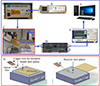 |
Figure 2 Schematic diagram illustrating the experimental setup for point contact excitation and detection. Signal generation (Block A) amplifies the signal (Block B), exciting the acoustic waves in the Coulomb probe configuration (Block C). The trans-impedance conversion (Block D) directs signals to the oscilloscope (Block E) for averaging and digitization. Subsequently, data is transferred via USB to a PC (Block F). Block G represents the probe and sample placement setup within the Faraday cage, while block C (highlighted with a red rectangle) schematically corresponds to block G, illustrating the sender and receiver probes. The image acquisition area was 10 mm × 10 mm, with a step size of 50 μm in both directions. |
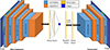 |
Figure 3 Example images showing the quality and diversity of generated images compared to real images. The generated images capture intricate details and variations, demonstrating the effectiveness of the proposed data augmentationtechnique. |
4 Image augmentation/generation by GAN
4.1 Original data set and curation for supervised learning
To facilitate the development and evaluation of the data augmentation technique, a dataset comprising spatiotemporal data matrices obtained through Coulomb coupling imaging was utilized. Each matrix has dimensions of 200 × 200 × 365, representing the spatial and temporal characteristics of the acquired data. Specifically, the spatial dimension of each snapshot corresponds to 200 pixels by 200 pixels, which is equivalent to a physical area of 10 mm × 10 mm. The dataset was collected by conducting experiments over a total acquisition time of 1 microsecond, resulting in 4000 time-varying snapshots. Notably, the images exhibit a repetitive pattern approximately every 365 snapshots, which reflects the periodic nature of the observed waves. This periodicity arises due to the specific experimental conditions, where the images capture the dynamic behavior of the material under investigation. To streamline the analysis, one complete cycle of 365 images was selected from the dataset, effectively encapsulating the unique wave patterns needed for model training and evaluation. This selection ensures that the dataset provides a comprehensive representation of the wave phenomena for detailed analysis. A comprehensive description of the experimental setup is provided in the following section. Subsequent sections will elaborate on the methodology and results obtained through the application of GANs to this distinctive Coulomb coupling imaging dataset. The use of GANs aims to enhance the data augmentation process, improving the robustness and accuracy of models trained on this spatiotemporal data.
4.2 Model architecture
GAN is formalized within a mathematical framework comprising two distinct neural networks – the Generator G and the Discriminator D. The primary objective of GANs is to learn a data distribution from training samples and subsequently generate synthetic data that closely mimics the distribution of the training set. The GAN framework is driven by a min–max game between G and D, where G strives to generate synthetic data to deceive D, and D endeavors to distinguish between real and synthetic samples. The adversarial training process involves optimizing the following objective function:
![Mathematical equation: $$ \begin{aligned} \min _{G}\ \max _{D}\ V\left( D,G \right)&=E_{x\sim p_{\rm data}(x)}\left[ \log D\left( x \right) \right]\nonumber \\&\quad +E_{z\sim p_{z}\left( z \right)}\left[ \log \left( 1-D\left( G\left( z \right) \right) \right) \right]. \end{aligned} $$](/articles/aacus/full_html/2025/01/aacus240115/aacus240115-eq2.gif) (2)
(2)
Here, x represents real samples from the data distribution pdata(x), and z is a latent variable sampled from a noise distribution pz(z). D(x) represents the output of the discriminator for real samples, while D(G(z))) denotes the output for synthetic samples generated by G.
4.2.1 Discriminator architecture
The Discriminator D within the GAN architecture is designed to classify the authenticity of input samples, distinguishing between real and synthetic Coulomb coupling images. To enhance the stability of the GAN training, we also incorporated spectral normalization, a regularization technique applied to the weights of each layer in D in the proposed methods. The spectral normalization is characterized by the following transformation for a weight matrix W [38]:
 (3)
(3)
where σ(W) denotes the largest singular value of W. The discriminator architecture involves multiple layers, each subject to spectral normalization. Following these layers, a dense layer is utilized for the final binary classification decision.
Let x represent the input Coulomb coupling image, and D(x) denote the discriminator’s output. The discriminator is trained to maximize the following objective function:
![Mathematical equation: $$ \begin{aligned} {\mathcal{L} }_{D}&={\mathbb{E} }_{x\sim p_{\rm data}(x)}[\log D(x)]\nonumber \\&\quad +{\mathbb{E} }_{z\sim p_{z}(z)}[\log (1-D(G(z)))] \end{aligned} $$](/articles/aacus/full_html/2025/01/aacus240115/aacus240115-eq4.gif) (4)
(4)
where pdata(x) is the distribution of real Coulomb coupling images, pz(z) represents the distribution of random noise z, and G(z) is the generator’s output.
The Discriminator is designed to classify input samples as real or synthetic. It incorporates multiple convolutional layers to capture spatial features effectively, followed by spectral normalization to stabilize training and prevent mode collapse. Spectral normalization, as shown in equation (3), constrains the largest singular value of the weight matrix, ensuring controlled weight scaling and improved gradient flow during backpropagation [38]. Each convolutional layer reduces spatial dimensions progressively while increasing feature depth to learn hierarchical representations. The final layers consist of dense connections for binary classification (Fig. 4).
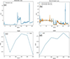 |
Figure 4 Schematic diagram representing the network architecture. This entire architecture represents the “Network Under Training” as shown in Figure 1. The network consists of two main components: a discriminator and a generator. The generator creates synthetic images from random noise, while the discriminator evaluates their authenticity against real images, facilitating the training process to improve image quality and diversity. |
4.2.2 Generator architecture
The Generator G is tasked with synthesizing realistic Coulomb coupling images from random noise. Leveraging the spatial dependency capturing capabilities of Convolutional Neural Networks (CNNs), we employ a CNN architecture for G. Let z denote the random noise vector sampled from pz(z), and G(z) represent the generator’s output. The generator architecture incorporates a series of convolutional layers, each followed by batch normalization and non-linear activation functions. This progressive refinement enables G to generate synthetic images that ideally resemble real Coulomb coupling images. The generator is trained to minimize the following objective function:
![Mathematical equation: $$ \begin{aligned} \mathcal{L} _{G}=\mathbb{E} _{z\sim p_{z}(z)}[\log (1-D(G(z)))]. \end{aligned} $$](/articles/aacus/full_html/2025/01/aacus240115/aacus240115-eq6.gif) (5)
(5)
This objective encourages G to produce synthetic images that D are classified as real. The GAN architecture is trained iteratively, with the generator and discriminator engaged in a dynamic interplay until convergence is achieved.
The Generator synthesizes Coulomb coupling images from random noise vectors sampled from pz(z). A CNN architecture is employed, leveraging its ability to learn spatial dependencies. The generator progressively upsamples the noise vector through transposed convolutional layers, adding depth and refining spatial resolution at each stage. Layers such as 4 × 4 × 512, 8 × 8 × 256, and 16 × 16 × 128 are standard in similar architectures like DCGAN [19, 39] and StyleGAN [40], ensuring a smooth transformation from low-resolution noise to high-resolution images. Each convolutional layer is followed by batch normalization, a technique that normalizes the output of the layer to ensure consistency and stability in the learning process. This helps accelerate training, reduce the sensitivity to initialization, and mitigate the risk of overfitting. Additionally, non-linear activation functions (e.g., ReLU, Rectified Linear Unit) are applied to introduce non-linearity into the model. This non-linearity is essential for the network to learn and represent complex patterns and features in the data, enhancing its ability to solve sophisticated tasks effectively.
4.3 Training strategy
The training strategy for the proposed GAN involves carefully tuning several hyperparameters to ensure optimal convergence and performance. The key hyperparameters include:
-
(1)
Noise Dimension z:z a latent variable sampled from a noise distribution and is an essential input to the generator. In this architecture, z is a vector of dimension 200.
-
(2)
Batch Size: the number of samples processed in each iteration. We set the batch size to 64, balancing computational efficiency and stability during training.
-
(3)
Image Dimensions: the width, height, and number of channels for the Coulomb coupling images. In this case, the images have dimensions of 200 × 200 pixels with a single channel.
-
(4)
Loss Function: we employ binary cross-entropy loss, suitable for binary classification problems, where the discriminator aims to distinguish between real and synthetic images.
-
(5)
Optimizer: Adam optimizer is chosen for its adaptive learning rate properties. The optimizer’s parameters are set as Adam(0.0002, 0.5), with a learning rate of 0.0002 and β1 set to 0.5.
In the initial step of training the discriminator, random batches comprising real Coulomb coupling images are systematically sampled from the dataset. Following this, the discriminator undergoes training to adeptly classify synthetic images with corresponding labels set to 0. This classification process involves the computation of binary cross-entropy loss. The culmination of these steps results in a combined discriminator loss, which, in turn, is utilized to update the weights of the discriminator. This iterative process ensures that the discriminator becomes increasingly proficient in distinguishing between real and synthetic images, enhancing the overall effectiveness of the model.
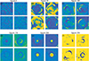 |
Figure 5 Performance metrics and loss trends during training. (a) Generator loss curve, showing the training progression of the generator over 250 epochs. (b) Discriminator loss curves for real and fake samples, reflecting the discriminator’s ability to distinguish between generated and real data. (c) PSNR values over epochs, illustrating the quality of the generated outputs. (d) SSIM values across epochs, indicating the structural fidelity of the generated images. |
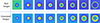 |
Figure 6 Images illustrating the visual quality of generated outputs at different training epochs. These images demonstrate the progression and improvement in image quality as the training process evolves, showing high-quality and diverse images at optimal epochs (a, b, c, and e). Additionally, the figure (f) includes examples of overfitted images generated at later epochs, highlighting the decrease in quality and diversity due to overfitting. |
On the other hand, in the training phase of the generator, the initial step involves the random sampling of noise vectors from the specified noise distribution. Subsequently, the generator undergoes training to produce synthetic images that the discriminator classifies as authentic, as denoted by D(G(z)) = 1. During this training, the binary cross-entropy loss is calculated to quantify the dissimilarity between the generated images and the real ones. The generator’s weights are then updated based on this adversarial loss, refining its ability to generate synthetic images that closely resemble real samples. This iterative process contributes to the continual improvement of the generator’s performance within the adversarial framework. The training of the discriminator and generator is repeated iteratively, allowing G and D to refine their strategies in an adversarial manner. The training continues until the desired convergence criteria are met, ensuring that G generates synthetic images that are indistinguishable from real ones according to D.
The training was conducted using an NVIDIA Tesla T4 GPU with 16 GB of memory, taking approximately 3 h to complete. Post-training, the model can generate data rapidly within seconds using random noise inputs. The generator model comprises 65 428 737 parameters, occupying 249.59 MB, while the discriminator model contains 677 249 parameters, occupying 2.58 MB. Notably, only the generator model is required during inference, significantly reducing computational overhead and enabling efficient data generation.
The model was trained for 200 epochs. It was observed that extending the training to 250 epochs resulted in overfitting, as illustrated in Figures 5 and 6, and Table 1. Figure 5 illustrates the performance metrics and loss trends during training: (a) the generator loss curve, showing its progression over 250 epochs; (b) discriminator loss curves for real and fake samples, reflecting the discriminator’s ability to differentiate between generated and real data; (c) PSNR values across epochs, indicating the quality of generated outputs; and (d) SSIM values over epochs, demonstrating the structural fidelity of the generated images. At 200 epochs, the model demonstrated the ability to generate high-quality and diverse images while effectively mitigating overfitting. This is evidenced by the high Structural Similarity Index Measure (SSIM) and Peak Signal-to-Noise Ratio (PSNR) scores observed at 200 epochs compared to other stages of training. The SSIM and PSNR values, calculated by comparing the generated images with the original images, highlight the model’s capacity to maintain structural fidelity and image quality. This optimal training duration ensures that the generated images retain variability and robustness without compromising quality.
SSIM and PSNR scores of the generated images as compared with the original images across different epochs at intervals of 50. We see that the model performance peaks at epoch 200 and then declines due to model overfitting.
5 Results evaluation
The evaluation of the GAN for synthesizing high-resolution Coulomb coupling images is grounded in quantitative metrics and visual comparisons. The primary metrics employed include the Wasserstein Distance, Jensen–Shannon Divergence, and Divergence Amongst Generated Images [41, 42].
5.1 Evaluation metrics
5.1.1 Wasserstein Distance
The Wasserstein Distance, also known as Earth Mover’s Distance (EMD), quantifies the dissimilarity between two probability distributions [41]. For context, it measures the discrepancy between the distribution of real Coulomb coupling images and the distribution of synthetic images generated by the GAN. Mathematically, the Wasserstein Distance is expressed as:
![Mathematical equation: $$ \begin{aligned} W(P_{r},P_{g})=\mathrm{inf}_{\gamma \in \mathrm \Pi (P_{r},P_{g})}\mathbb{E} _{(x,y)\sim \gamma }[\Vert x-y\Vert ] \end{aligned} $$](/articles/aacus/full_html/2025/01/aacus240115/aacus240115-eq7.gif) (6)
(6)
where Pr is the distribution of real images, Pg is the distribution of generated images, and γ is the set of all joint distributions over real and generated samples that have marginals Pr and Pg. In this case, we employ Wasserstein distance between real and generated datasets. Ideally the distributions of these datasets should be close to each other (and hence low Wassersteindistance).
Evaluation Metrics for Different Methods. Lower values for Wasserstein Distance and Jensen–Shannon Divergence indicate better performance, while a higher value for Divergence Amongst Generated Images signifies greater diversity.
5.1.2 Jensen–Shannon Divergence
The Jensen–Shannon Divergence measures the similarity between two probability distributions. In this case, it quantifies the dissimilarity between the distribution of real Coulomb coupling images and the distribution of synthetic images generated by the GAN. Mathematically, the Jensen–Shannon Divergence is calculated as:
 (7)
(7)
where DKL is the Kullback–Leibler Divergence, Pr is the distribution of real images, Pg is the distribution of generated images, and M is the midpoint distribution. We calculate the Jensen–Shannon divergence between the real and generated datasets. A good GAN model should be able to generate datasets whose distribution is close to that of the real dataset (and hence low Jensen–Shannon divergence).
5.1.3 Image diversity
This metric evaluates the diversity among the generated images, helping to assess how varied the synthetic images are in terms of capturing different features and patterns [43]. The diversity is calculated using Jensen–Shannon Divergence, a method that measures the similarity between two probability distributions. In this context, the Jensen–Shannon Divergence is applied between pairs of generated images to quantify their diversity. High image diversity indicates that the GAN model can generate a wide range of images with different characteristics, which is crucial for creating a robust and comprehensive dataset. This diversity ensures that the model does not produce repetitive or overly similar images, thereby enhancing the overall quality and usefulness of the generated data for training purposes. Ideally, the image diversity should be high, signifying the GAN model’s ability to produce diverse images that accurately reflect the variability in real-world data. This helps improve the model’s generalization capabilities, making it more effective in various applications.
5.2 Results
As shown in Table 1, the SSIM and PSNR values vary as the number of epochs increases, indicating the impact of training duration on image quality. Figure 6 provided a visual representation of how the quality of the generated images improves with more epochs. To further elaborate, Table 2 presents the metrics for different methods, while Figure 3 showcases example images from both the real and generated datasets, offering a comparison and deeper insights into the model’s performance.
The metrics demonstrate the efficacy of the GAN in capturing the distribution of real images and the diversity in the generated dataset. Although pixel-level transformation generates data whose distribution is closer to the real data distribution, these transformations have the limitation that only a limited number of data can be generated. The proposed method and its training variations outperform the traditional data augmentation techniques across 2 of the 3 metrics, namely Jensen–Shannon divergence and image diversity. Note that “Proposed method + ADA” signifies the proposed method trained using the AdaBoost algorithm [44].
Lower Wasserstein Distance (WD) values indicate better alignment between generated and real datasets. Pixel-level transformations achieve the lowest WD (0.11), but such low values often result in reduced diversity in the generated data. The proposed method achieves a balanced WD of 0.27, generating realistic data while maintaining diversity. Similarly, the Jensen–Shannon Divergence (JSD) value of 0.35 for the proposed method demonstrates strong alignment with real data, outperforming traditional methods like affine transformations, which have a higher JSD of 0.56 and fail to capture dataset complexities. Research on GAN performance highlights that lower divergence values signify a model’s ability to accurately represent the real data distribution [45]. In terms of diversity, the “Proposed Method + ADA” achieves the highest Image Diversity (ID) score of 0.84. This underscores the effectiveness of adaptive training techniques in generating varied and realistic samples. The visual examples further the quality and diversity achieved by the proposed GAN. The generated images exhibit intricate patterns and features akin to the real dataset, affirming that the proposed approach can synthesize high-resolution Coulomb coupling images for data augmentation in various research domains. The variations in the generated dataset reflect the variations present in the original dataset which consisted of time-varying snapshots.
6 Conclusion
This study demonstrates how GANs can effectively generate high-resolution images of Coulomb coupling, representing their potential in addressing complex imaging challenges. The designed GAN architecture delivers promising results, with low Wasserstein Distance and Jensen–Shannon Divergence values indicating a close alignment between real and generated images. These metrics validate the accuracy and reliability of the synthetic data produced by the model. In addition to accuracy, the significant divergence observed among the generated images highlights the model’s ability to create a diverse synthetic dataset. This diversity is essential for capturing a wide range of variations that closely resemble real-world scenarios, ensuring that the synthetic data can be effectively used in downstream applications. Such diverse datasets have a profound impact on data augmentation strategies, enabling more robust and comprehensive investigations across various domains, including biomedical imaging and materials science. By providing high-quality synthetic datasets, GANs can fill gaps in experimental data, reduce dependency on costly and time-intensive data collection processes, and support the development of innovative solutions. Furthermore, the ability to generate realistic and diverse datasets enhances the accuracy and robustness of computational models, allowing them to better represent the variability seen in real-world conditions. This study highlights the utility of GANs as a powerful tool for scientific research, paving the way for more effective data-driven approaches in fields requiring high-resolution and diverse imaging data.
Conflicts of interest
All authors declare no conflict of interest.
Data availability statement
The methods discussed in this paper are available in GitHub, under the reference [12].
References
- N.M. Kalimullah, A. Shelke, A. Habib: A deep learning approach for anomaly identification in PZT sensors using point contact method. Smart Materials and Structures 32, 9 (2023) 095027. [CrossRef] [Google Scholar]
- N.M. Kalimullah, K. Shukla, A. Shelke, A. Habib: Stiffness tensor estimation of anisotropic crystal using point contact method and unscented Kalman filter. Ultrasonics 131 (2023) 106939. [CrossRef] [PubMed] [Google Scholar]
- M. Pluta, M. von Buttlar, A. Habib, E. Twerdowski, R. Wannemacher, W. Grill: Modeling of Coulomb coupling and acoustic wave propagation in LiNbO3. Ultrasonics 48, 6, 7 (2008) 583–586. [CrossRef] [PubMed] [Google Scholar]
- V. Agarwal, A. Shelke, B.S. Ahluwalia, F. Melandsø, T. Kundu, A. Habib: Damage localization in piezo-ceramic using ultrasonic waves excited by dual point contact excitation and detection scheme. Ultrasonics 108 (2020) 106113. [CrossRef] [PubMed] [Google Scholar]
- A. Habib, A. Shelke, M. Pluta, U. Pietsch, T. Kundu, W. Grill: Scattering and attenuation of surface acoustic waves and surface skimming longitudinal polarized bulk waves imaged by Coulomb coupling, in: AIP Conference Proceedings. American Institute of Physics, 2012. [Google Scholar]
- A. Habib, E. Twerdowski, M. von Buttlar, M. Pluta, M. Schmachtl, R. Wannemacher, W. Grill: Acoustic holography of piezoelectric materials by Coulomb excitation, in: Health Monitoring and Smart Nondestructive Evaluation of Structural and Biological Systems V. SPIE, 2006. [Google Scholar]
- H. Singh, A.S. Ahmed, F. Melandsø, A. Habib: Ultrasonic image denoising using machine learning in point contact excitation and detection method. Ultrasonics 127 (2023) 106834. [CrossRef] [PubMed] [Google Scholar]
- S. Jadhav, R. Kuchibhotla, K. Agarwal, A. Habib, D.K. Prasad: Deep learning-based denoising of acoustic images generated with point contact method. Journal of Nondestructive Evaluation, Diagnostics and Prognostics of Engineering Systems 6, 3 (2023) 031002. [CrossRef] [Google Scholar]
- P. Banerjee, P. Saxena, N.M. Kalimullah, A. Shelke, A. Habib: Damage detection and localization by learning deep features of elastic waves in piezoelectric ceramic using point contact method, in: Proceedings of the IEEE/CVF Conference on Computer Vision and Pattern Recognition, 2024. [Google Scholar]
- Y. Shen, J. Liang, M.C. Lin: Gan-based garment generation using sewing pattern images, in: Computer Vision–ECCV 2020: 16th European Conference, Glasgow, UK, August 23–28, 2020, Proceedings, Part XVIII 16. Springer, 2020. [Google Scholar]
- F. Garcea, A. Serra, F. Lamberti, L. Morra: Data augmentation for medical imaging: a systematic literature review. Computers in Biology and Medicine 152 (2023) 106391. [CrossRef] [PubMed] [Google Scholar]
- P. Banerjee, et al.: Data set used in this manuscript, in: banerjeepragyan/DataAugmentation. GitHub, 2024. https://github.com/banerjeepragyan/DataAugmentation. [Google Scholar]
- S.J.N. Anita, C.J. Moses: Survey on pixel level image fusion techniques, in: 2013 IEEE International Conference ON Emerging Trends in Computing, Communication and Nanotechnology (ICECCN). IEEE, 2013. [Google Scholar]
- S. Liu, J. Zhang, Y. Chen, Y. Liu, Z. Qin, T. Wan: Pixel level data augmentation for semantic image segmentation using generative adversarial networks, in: ICASSP 2019-2019 IEEE International Conference on Acoustics, Speech and Signal Processing (ICASSP). IEEE, 2019. [Google Scholar]
- A. Laugros, A. Caplier, M. Ospici: Addressing neural network robustness with mixup and targeted labeling adversarial training, in: Computer Vision–ECCV 2020 Workshops: Glasgow, UK, August 23–28, 2020, Proceedings, Part V 16. Springer, 2020. [Google Scholar]
- C. Shorten, T.M. Khoshgoftaar: A survey on image data augmentation for deep learning. Journal of Big Data 6, 1 (2019) 1–48. [CrossRef] [Google Scholar]
- K. Wang, C. Gou, Y. Duan, Y. Lin, X. Zheng, F.Y. Wang: Generative adversarial networks: introduction and outlook. IEEE/CAA Journal of Automatica Sinica 4, 4 (2017) 588–598. [CrossRef] [Google Scholar]
- M. Frid-Adar, I. Diamant, E. Klang, M. Amitai, J. Goldberger, H. Greenspan: GAN-based synthetic medical image augmentation for increased CNN performance in liver lesion classification. Neurocomputing 321 (2018) 321–331. [CrossRef] [Google Scholar]
- A. Radford, L. Metz, S. Chintala: Unsupervised representation learning with deep convolutional generative adversarial networks. Preprint https://arxiv.org/abs/1511.06434, 2015. [Google Scholar]
- E.L. Denton, S. Chintala, R. Fergus: Deep generative image models using aOBJ Laplacian pyramid of adversarial networks. Advances in Neural Information Processing Systems (2015) 28. [Google Scholar]
- M. Mirza, S. Osindero: Conditional generative adversarial nets. Preprint https://arxiv.org/abs/1411.1784, 2014. [Google Scholar]
- A. Odena, C. Olah, J. Shlens: Conditional image synthesis with auxiliary classifier gans, in: International Conference on Machine Learning. PMLR, 2017. [Google Scholar]
- P. Isola, J.Y. Zhu, T. Zhou, A.A. Efros: Image-to-image translation with conditional adversarial networks, in: Proceedings of the IEEE Conference on Computer Vision and Pattern Recognition, 2017. [Google Scholar]
- A. Antoniou, A. Storkey, H. Edwards: Data augmentation generative adversarial networks. Preprint https://arxiv.org/abs/1711.04340, 2017. [Google Scholar]
- V. Sandfort, K. Yan, P.J. Pickhardt and R.M. Summers: Data augmentation using generative adversarial networks (CycleGAN) to improve generalizability in CT segmentation tasks. Scientific Reports 9, 1 (2019) 16884. [CrossRef] [PubMed] [Google Scholar]
- O. Ronneberger, P. Fischer, T. Brox: U-net: convolutional networks for biomedical image segmentation, in: Medical Image Computing and Computer-Assisted Intervention–MICCAI 2015: 18th International Conference, Munich, Germany, October 5–9, 2015, Proceedings, Part III 18. Springer, 2015. [Google Scholar]
- E. Wu, K. Wu, D. Cox, W. Lotter: Conditional infilling GANs for data augmentation in mammogram classification, in: Image Analysis for Moving Organ, Breast, and Thoracic Images: Third International Workshop, RAMBO 2018, Fourth International Workshop, BIA 2018, and First International Workshop, TIA 2018, Held in Conjunction with MICCAI. Springer, Granada, Spain, 2018. [Google Scholar]
- G. Cohen, S. Afshar, J. Tapson, A. Van Schaik: EMNIST: extending MNIST to handwritten letters, in: 2017 International Joint Conference on Neural Networks (IJCNN). IEEE, 2017. [Google Scholar]
- Z. Qawaqneh, A.A. Mallouh, B.D. Barkana: Deep convolutional neural network for age estimation based on VGG-face model. Preprint https://arxiv.org/abs/1709.01664, 2017. [Google Scholar]
- S. Fabi, S. Otte, F. Scholz, J. Wührer, M. Karlbauer, M.V. Butz: Extending the omniglot challenge: imitating handwriting styles on a new sequential data set. IEEE Transactions on Cognitive and Developmental Systems 15, 2 (2022) 896–903. [Google Scholar]
- T. Yao, C. Qu, Q. Liu, R. Deng, Y. Tian, J. Xu, A. Jha, S. Bao, M. Zhao, A. Fogo: Deep Generative Models, and Data Augmentation, Labelling, and Imperfections. Springer, Cham, Switzerland, 2021. [Google Scholar]
- A. Shelke, A. Habib, U. Amjad, M. Pluta, Tribikram Kundu, U. Pietsch, W. Grill: Metamorphosis of bulk waves to Lamb waves in anisotropic piezoelectric crystals, in: Health Monitoring of Structural and Biological Systems 2011. SPIE, 2011. [Google Scholar]
- A. Habib, U. Amjad, M. Pluta, U. Pietsch, W. Grill: Surface acoustic wave generation and detection by Coulomb excitation, in: Health Monitoring of Structural and Biological Systems 2010. SPIE, 2010. [Google Scholar]
- N.M. Kalimullah, A. Shelke, A. Habib: Multiresolution dynamic mode decomposition (mrDMD) of elastic waves for damage localisation in piezoelectric ceramic. IEEE Access 9 (2021) 120512–120524. [CrossRef] [Google Scholar]
- A. Habib, E. Twerdowski, M. von Buttlar, R. Wannemacher, W. Grill: The influence of the radius of the electrodes employed in Coulomb excitation of acoustic waves in piezoelectric materials, in: Health Monitoring of Structural and Biological Systems 2007. SPIE, 2007. [Google Scholar]
- E. Jacobsen: Sources of sound in piezoelectric crystals. The Journal of the Acoustical Society of America 32, 8 (1960) 949–953. [CrossRef] [Google Scholar]
- R. Pal, N. Ghosh, N.M. Kalimullah, A. Ahmad, F. Melandsø, A. Habib: Subsurface damage identification and localization in PZT ceramics using point contact excitation and detection: an image processing framework. Ultrasonics 147 (2024) 107516. [Google Scholar]
- T. Miyato, T. Kataoka, M. Koyama, Y. Yoshida: Spectral normalization for generative adversarial networks. Preprint https://arxiv.org/abs/1802.05957, 2018. [Google Scholar]
- C. Dewi, R.C. Chen, Y.T. Liu, S.K. Tai: Synthetic Data generation using DCGAN for improved traffic sign recognition. Neural Computing and Applications 34, 24 (2022) 21465–21480. [CrossRef] [Google Scholar]
- T. Karras, S. Laine, M. Aittala, J. Hellsten, J. Lehtinen, T. Aila: Analyzing and improving the image quality of stylegan, in: Proceedings of the IEEE/CVF Conference on Computer Vision and Pattern Recognition, 2020. [Google Scholar]
- V.M. Panaretos, Y. Zemel: Statistical aspects of Wasserstein distances. Annual Review of Statistics and its Application 6, 1 (2019) 405–431. [CrossRef] [Google Scholar]
- M.L. Menéndez, J.A. Pardo, L. Pardo, M.C. Pardo: The Jensen–Shannon divergence. Journal of the Franklin Institute. 334, 2 (1997) 307–318. [CrossRef] [MathSciNet] [Google Scholar]
- H.-Y. Lee, H.Y. Tseng, J.B. Huang, M. Singh, M.H. Yang: Diverse image-to-image translation via disentangled representations, in: Proceedings of the European Conference on Computer Vision (ECCV), 2018. [Google Scholar]
- Y. Freund, R.E. Schapire: A decision-theoretic generalization of on-line learning and an application to boosting. Journal of Computer and System Sciences 55, 1 (1997) 119–139. [Google Scholar]
- M. Arjovsky, L. Bottou: Towards principled methods for training generative adversarial networks. Preprint https://arxiv.org/abs/1701.04862, 2017. [Google Scholar]
Cite this article as: Banerjee P. Ojha S. Kalimullah N.M.M. Shelke A. & Habib A. 2025. Ultrasonic wave field image augmentation in PZT sensors using generative machine learning and Coulomb coupling. Acta Acustica, 9, 15. https://doi.org/10.1051/aacus/2025002.
All Tables
SSIM and PSNR scores of the generated images as compared with the original images across different epochs at intervals of 50. We see that the model performance peaks at epoch 200 and then declines due to model overfitting.
Evaluation Metrics for Different Methods. Lower values for Wasserstein Distance and Jensen–Shannon Divergence indicate better performance, while a higher value for Divergence Amongst Generated Images signifies greater diversity.
All Figures
|
Figure 1 This figure depicts the overall strategy used in this paper. First, real data (ground truth) is acquired. This is followed by GAN-based data augmentation. Real images and random noise input images are fed into the network used to train. The network output is further used as error back-propagation to train the network. |
| In the text | |
|
Figure 2 Schematic diagram illustrating the experimental setup for point contact excitation and detection. Signal generation (Block A) amplifies the signal (Block B), exciting the acoustic waves in the Coulomb probe configuration (Block C). The trans-impedance conversion (Block D) directs signals to the oscilloscope (Block E) for averaging and digitization. Subsequently, data is transferred via USB to a PC (Block F). Block G represents the probe and sample placement setup within the Faraday cage, while block C (highlighted with a red rectangle) schematically corresponds to block G, illustrating the sender and receiver probes. The image acquisition area was 10 mm × 10 mm, with a step size of 50 μm in both directions. |
| In the text | |
|
Figure 3 Example images showing the quality and diversity of generated images compared to real images. The generated images capture intricate details and variations, demonstrating the effectiveness of the proposed data augmentationtechnique. |
| In the text | |
|
Figure 4 Schematic diagram representing the network architecture. This entire architecture represents the “Network Under Training” as shown in Figure 1. The network consists of two main components: a discriminator and a generator. The generator creates synthetic images from random noise, while the discriminator evaluates their authenticity against real images, facilitating the training process to improve image quality and diversity. |
| In the text | |
|
Figure 5 Performance metrics and loss trends during training. (a) Generator loss curve, showing the training progression of the generator over 250 epochs. (b) Discriminator loss curves for real and fake samples, reflecting the discriminator’s ability to distinguish between generated and real data. (c) PSNR values over epochs, illustrating the quality of the generated outputs. (d) SSIM values across epochs, indicating the structural fidelity of the generated images. |
| In the text | |
|
Figure 6 Images illustrating the visual quality of generated outputs at different training epochs. These images demonstrate the progression and improvement in image quality as the training process evolves, showing high-quality and diverse images at optimal epochs (a, b, c, and e). Additionally, the figure (f) includes examples of overfitted images generated at later epochs, highlighting the decrease in quality and diversity due to overfitting. |
| In the text | |
Current usage metrics show cumulative count of Article Views (full-text article views including HTML views, PDF and ePub downloads, according to the available data) and Abstracts Views on Vision4Press platform.
Data correspond to usage on the plateform after 2015. The current usage metrics is available 48-96 hours after online publication and is updated daily on week days.
Initial download of the metrics may take a while.