| Issue |
Acta Acust.
Volume 9, 2025
|
|
|---|---|---|
| Article Number | 61 | |
| Number of page(s) | 16 | |
| Section | Building Acoustics | |
| DOI | https://doi.org/10.1051/aacus/2025050 | |
| Published online | 17 October 2025 | |
Scientific Article
An outdoor-to-indoor sound propagation modelling framework for evaluating noise exposure applications
Building Acoustics Group, Department of the Built Environment, Eindhoven University of Technology, Het Kranenveld 8, Eindhoven, 5612 AZ, The Netherlands
* Corresponding author: This email address is being protected from spambots. You need JavaScript enabled to view it.
Received:
5
June
2025
Accepted:
11
September
2025
Abstract
Environmental noise exposure has shown to have significant negative effects on people’s lives. In noise exposure studies, outdoor noise levels are usually preferred over indoor levels for investigating exposure-response relationships, introducing a systematic risk of bias. Hence, an outdoor-to-indoor sound propagation modelling framework is defined for estimating indoor noise levels based on outdoor levels. Particularly, by expressing outdoor and indoor sound propagation via energetic models and façade (multi-component and multi-layered) structures via computational sound insulation models (Transfer Matrix Method), outdoor-based indoor impulse responses can be generated. To validate the framework, a case study was conducted, showing that measured and simulated sound insulation were in good agreement. Finally, this framework was applied to generate datasets of outdoor and indoor noise levels (noise indicators) based on scenarios of outdoor environment, indoor environment, and façade structures. This allows the training of statistical learning approaches for estimating indoor noise levels and identifying important predictors. Results show that a random-forest approach outperforms a stepwise and a neural network approach across all the employed noise indicators (RMSE < 2 dB). These models enable the estimation of indoor sound exposure levels based on outdoor levels as well as the exploration of exposure-response relationships in locations with known built environment characteristics.
Key words: Sound insulation / Sound propagation / Impulse response synthesis / Noise exposure / Statistical learning
© The Author(s), Published by EDP Sciences, 2025
 This is an Open Access article distributed under the terms of the Creative Commons Attribution License (https://creativecommons.org/licenses/by/4.0), which permits unrestricted use, distribution, and reproduction in any medium, provided the original work is properly cited.
1 Introduction
Exposure to urban noise has shown significant negative effects on people’s health [1–4]. Annoyance [1, 5, 6], quality of life [7, 8], and a range of cardiometabolic outcomes [3, 9, 10] are some of the most studied noise-induced health effects. Chronic noise exposure during the children’s developmental period (mental and physical) may be responsible for the presence of harmful health effects in later life [3, 11]. However, in studies of noise exposure [4], noise-induced health effects are primarily investigated with respect to outdoor noise exposure levels as opposed to indoor levels. This suggests the presence of a systematic risk of bias in the explored exposure-response relationship between indoor noise exposure levels and health outcomes. This would be particularly evident in the case of vulnerable groups (e.g., children and elderly) who spend the majority of their time indoors [12].
In outdoor-to-indoor sound propagation, façade structures can be considered as a key aspect [4]. Various methodologies have been proposed for the calculation of sound insulation in monolithic structures, encompassing numerical and analytical techniques [13]. Concerning analytical approaches, closed-form solutions have been derived for single-layered [14–17] and double-layered [15, 17, 18] structures. Among the various numerical modelling approaches, the Finite Element Method [19] (FEM) and the Boundary Element Method [20] (BEM) correspond to powerful yet complex calculation methodologies. The TMM can be regarded as an alternative approach, particularly well-suited to the efficient calculation of the sound insulation of multi-layered structures of infinite size [21, 22]. The TMM can provide a good approximation in the mid to high frequency range [13]. However, at lower frequencies, where the structures display a strong modal behaviour, the accuracy is reduced [13]. The impact of the finite dimensions of the structures on the modelling of sound transmission can be approached through the use of the spatial windowing technique [23]. This technique is based on the radiation efficiency of rectangular structures [23–28], reducing the uncertainties at lower frequencies. Considering rectilinear surfaces (e.g., rectangular surface, accompanied by a rectangular aperture), a methodology has recently been proposed to calculate radiation efficiency [29]. This approach entails the sub-division of the rectilinear surface into a number of rectangular sub-surfaces, with the radiation efficiency of each sub-surface being calculated. In TMM, the effect of studs can also be incorporated, depending on the structure and connection type [30–33].
For the assessment of noise propagation from outdoors to indoors, synchronised noise exposure measurements are typically carried out based on supervised [34] or unsupervised [35, 36] approaches, while noise exposures are primarily expressed via the A-weighted equivalent noise indicator (L Aeq). To estimate outdoor-to-indoor level differences, statistical prediction modelling techniques (e.g. regression models) have been employed [34, 36]. These techniques take into account outdoor noise exposure levels and factors related to both outdoor and indoor environments, as well as building façade characteristics. Alternatively, single-valued outdoor-to-indoor attenuationfactors provide a simplified approach for the correction of outdoor noise exposure levels [34, 36–39]. However, these techniques are particularly sensitive to study design characteristics (e.g., type of sound source, location of sound equipment, façade structure, and indoor acoustic conditions) and require a large number of measurements.
Computational modelling techniques (for auralization purposes) have been employed for the detailed characterization of the propagation of sound from outdoors to indoors via façade structures [40, 41]. Particularly, these techniques allow for synthesizing outdoor-based indoor impulse responses, taking into account the characteristics of both outdoor and indoor environments as well as building façade structures. However, they are constrained to monolithic single-leaf façade structures, where sound insulation is calculated via analytical formulae [40, 41]. This limitation is particularly noteworthy given the prevalence of multi-leaf structures (e.g., double-leaf walls or windows) in architectural designs. TMM is one alternative method that has not yet been applied to the calculation of sound insulation of multi-layered and multi-component structures in outdoor-to-indoor models.
When comparing the computational modelling techniques for auralization purposes and statistical modelling approaches, several key distinctions can be identified. The auralization-based computational modelling technique enables a detailed characterization of angle-dependent outdoor-to-indoor sound propagation through façade structures composed of multi-layered and multi-component surfaces with the aim of synthesizing outdoor-based indoor impulse responses. This denotes the difference in relation to other approaches such as in ISO 12354-3:2017 [42]. This facilitates the generation of simulation datasets for scenarios in which in-situ measurements are challenging or infeasible, and the conduction of psychoacoustic experiments. Conversely, statistical modelling techniques offer a simplified, data-driven means of representing outdoor-to-indoor sound propagation. These models rely on measured or predicted outdoor and indoor noise levels, along with additional predictors (e.g., environmental and building characteristics) that describe the outdoor-to-indoor sound propagation concept. In essence, the computational modelling framework provides a physically grounded, acoustics-driven methodology based on the understanding of sound propagation mechanisms and façade behaviour. In contrast, the statistical modelling framework supports an intuition-guided estimation of transmission effects through empirical data and prediction methods. Overall, the integration of computational modelling framework in dataset generation has the potential to improve the interpretability and reliability of statistical modelling framework. This is due to the controlled and detailed characterization of outdoor-to-indoor sound propagation pathways provided by the computational models, which offers a robust and physically informed basis for data synthesis.
The objective of this study is divided into two parts. In the first part, a computational modelling framework is defined to simulate the propagation of sound from outdoors to indoors through facade structures. In this framework, TMM is applied for the modelling of multi-layered structures, while the implementation of adjusted radiation efficiency allows for incorporating the design characteristics of multi-component structures. The validation of the computational modelling framework was performed through experimental measurements on a multi-component, multi-layered façade structure, with emphasis on its sound reduction index. In the second part, datasets based on various scenarios are generated using the computational modelling framework to estimate indoor noise levels (expressed by noise indicators) through statistical learning approaches with predictors related to outdoor levels, outdoor environment, indoor environment, and building façade structures. In the context of noise exposure studies, this study has the potential to simulate a wide range of built environments, making it possible to estimate indoor exposure levels on the basis of e.g., noise maps for outdoor sound levels and to assess the importance of different built environment characteristics, as well as to explore exposure-response relationships with respect to outdoor-based indoor noise exposure levels.
The structure of this work is as follows: Section 2 presents the façade sound insulation modelling. Sections 3 and 4 describe the outdoor-to-indoor propagation modelling and its implementation in estimating indoor noise levels through the utilization of statistical learning methodologies based on datasets generated via the propagation models, respectively. Section 5 presents and discusses the developed framework, including its validation and application. Section 6 summarises the main aspects.
2 Sound insulation modelling
For sound insulation modelling, TMM is applied [22]. The general principle of the TMM applied to an N-leaf structure is expressed in the following way. A plane wave impinges on the first layer of a material of thickness h 1 under an angle of incident θ (i.e., the angle between the direction of propagation of the incident plane wave and the normal to the plane of the layer) and propagates into the fluid cavity f, of depth d 1, and then to a second layer of a material, and so on, up to the last layer where the transmitted sound is radiated.
Considering an incident plane wave, the wave number component (parallel to the interface) k t of the incident wave in the free air can be expressed as [22] k t = k 0sin(θ), where k 0 denotes the wave number in free air. Hence, the sound propagation in a layer can be described by a transfer matrix [T] as V ( M ) = [T]V ( M ′ ), where V ( ⋅ ) denotes a vector whose components describe the acoustic field variables (sound pressure and particle velocity) at a point on the forward ( M ) and backward face ( M ′ ) of the layer, respectively.
2.1 Infinite-size sound transmission coefficient
For multi-layered structures subject to the thin-plate theory, a simple multiplication among the transfer matrices of various layers denotes the sound transmission coefficient [21, 22]. Using the definition of the transmission coefficient, the incident sound transmission coefficient of an infinite-sized structure with N leafs can be expressed as
 (1)
(1)
where the T inc, T p, T f, and T rad denote the transfer matrices of the incident, thin-plate, fluid, and radiated layer, respectively, as these are presented in, for example, [22].
For structures comprising heterogeneous layers, such as the combination of solid, fluid, poroelastic, and thin layers, it has been demonstrated that the aforementioned approach of computing the infinite sound transmission coefficient by multiplying transfer matrices is not applicable [22]. As a result, coupling interface matrices, which satisfy the continuity conditions between adjacent (transfer matrix) layers (as presented, e.g., in [22]) have been employed to facilitate the calculation of sound transmission coefficient in complex multi-layered structures via a global matrix, taking into account semi-infinite fluid conditions at the radiating surface.
For both thin- and heterogeneous-layered structures, the infinite sound reduction index of multi-layered structure under an angle of incidence θ can be expressed as [22]
 (2)
(2)
2.2 Spatial windowing technique
To account for the impact of finite surface dimensions on the sound transmission coefficient, a spatial windowing technique based on radiation efficiency can be employed [23]. Among the various methods proposed for computing the radiation efficiency of a rectangular plate (e.g. [23, 26, 27]), a computationally efficient approach was recently proposed in [28], requiring only a single integration (instead of a quadruple integration). This is expressed as [28]:
![Mathematical equation: $$ \begin{aligned} \sigma (k_\text{ p})&= \mathfrak{Re} \Bigg \{ \dfrac{2\text{ j}k_0}{\pi S}\int _{0}^{L_y} \Bigg ( \dfrac{L_xL_y\pi }{2}-L_yR-L_xR \nonumber \\&\quad \quad \quad \quad + \dfrac{R^2}{2} \Bigg )J_0(k_\text{ p}R)e^{-\text{ j}k_0R}\text{ d}R\Bigg \} \nonumber \\&+ \mathfrak{Re} \Bigg \{ \dfrac{2\text{ j}k_0}{\pi S} \int _{L_y}^{L_x} \Bigg ( L_xL_y\arcsin {\Bigg ( \dfrac{L_y}{2} \Bigg )} -\dfrac{L_y^2}{2} \nonumber \\&\quad \quad \quad \quad + L_x\sqrt{R^2-L_y^2}-L_xR \Bigg )J_0(k_\text{ p}R)e^{-\text{ j}k_0R}\text{ d}R \Bigg \} \nonumber \\&+ \mathfrak{Re} \Bigg \{ \dfrac{2\text{ j}k_0}{\pi S} \int _{L_x}^{\sqrt{L_x^2+L_y^2}} \Bigg [ L_xL_y \Bigg ( \arcsin {\Bigg (\dfrac{L_y}{R}\Bigg )} \nonumber \\&\quad \quad \quad \quad -\arccos {\Bigg (\dfrac{L_x}{R}\Bigg )} \Bigg ) + L_y\sqrt{R^2-L_x^2} \nonumber \\&+ L_x\sqrt{R^2-L_y^2}-\dfrac{L_x^2+L_y^2+R^2}{2} \Bigg ] J_0(k_\text{ p}R)e^{-\text{ j}k_0R}\text{ d}R \Bigg \}, \end{aligned} $$](/articles/aacus/full_html/2025/01/aacus250070/aacus250070-eq3.gif) (3)
(3)
where L
x
and L
y
denote the length and height of rectangular surfaces, S denotes the surface area, k
p denotes the wave-number of the plate, J
0 denotes the first order Bessel function, and ℜ𝔢{⋅} denotes the real-part of complex numbers with imaginary unit  .
.
To calculate the radiation efficiency of rectilinear surfaces (i.e., polygonal surfaces with sides intersecting at right angles), a method was recently proposed [29]. In this approach, rectilinear surfaces are divided into a set of isolated sub-surfaces, from which the radiation efficiency of each sub-surface is individually computed. To ensure continuity between adjacent sub-surfaces, their first-order correlation is incorporated, enabling the calculation of the radiation efficiency for each pair of adjacent sub-surfaces as a coupled system. A graphical illustration of the discretization of a rectilinear surface in isolated and adjacent surfaces is presented in Figure 1. Mathematically, the adjusted radiation efficiency can be formulated as [29]:
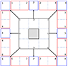 |
Figure 1 Discretization of a rectilinear surface (black shape outline) into isolated (blue shape outline) and adjacent (red shape outline) sub-surfaces. |
 (4)
(4)
where i and j denote the two adjacent sub-surfaces, S i and S j denote the areas of the isolated sub-surfaces i and j, N ϵ i denotes the number of adjacent elements ϵ i , and σ i j (k p) and σ i (k p) denote the radiation efficiency of adjacent i j and isolated i sub-surfaces calculated via equation (3).
A rectilinear surface was considered for the evaluation of the first-order adjusted radiation efficiency from equation (4) compared to numerical integration as in [28]. Specifically, a 3 m × 3 m glass surface, with material properties and plate wavenumber as in [29] were considered for evaluating the adjusted radiation efficiency. The results are illustrated in Figure 2. As it is shown, the first-order adjusted radiation efficiency σ(1)(kp) for the glazing surface exhibits strong agreement with the reference radiation efficiency σ(kp), particularly within the typical sound insulation frequency range of 50 Hz to 5 kHz. When focusing on the zeroth-order approximation σ(0)(kp), corresponding to the summation of the radiation efficiencies of isolated sub-surfaces while neglecting first-ordercorrelations between adjacent elements, a noticeable deviation from the reference curve was observed. This discrepancy highlights the importance of accounting for first-order correlation between adjacent sub-surfaces in the calculation of radiation efficiency. As highlighted in [29], a higher degree of correlation between adjacent surfaces must be accounted for when higher-order discretizations are employed. In the present study, a first-order discretization in conjunction with a first-order correlation has been considered.
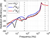 |
Figure 2 Adjusted radiation efficiency of a rectilinear glazing surface, computed using the zeroth-order σ(0)(kp) (blue) and first-order σ(1)(kp) (red) adjusted radiation efficiency, along with the numerically integrated reference curve σ(kp) (black). The gray dashed lines represent the typical frequency range in building acoustics, spanning from 50 Hz to 5 kHz. |
2.3 Finite-size sound transmission coefficient
By applying the spatial window to the infinite incident sound transmission coefficient, the finite incident sound transmission coefficient of a multi-layered rectangular structure can be obtained, expressed as [24, 25]:
 (5)
(5)
Similarly, the finite incident sound transmission coefficient for rectilinear surfaces can be expressed as [29]:
 (6)
(6)
where θ denotes all the angles of incidence to the isolated (θi) and the adjacent (θij) surfaces.
Finally, the finite incident sound reduction index R fin(θ) for both structures can be calculated as in equation (2).
2.4 Bridge connection
The effect of bridge connection (line or point) can additionally be incorporated to the finite sound transmission coefficient for double-leaf structures [30]. This is determined by the ratio between the power radiated from the second plate without the bridges only (W P, 2) and the power radiated as a result of the bridges (W B, 2). Assuming that the two contributions to the radiated power are uncorrelated, the finite sound reduction index, including the bridge connection, is expressed as [30]:
 (7)
(7)
where the impact of the bridge connection (i.e., the second term on the right-hand side of (Eq. 7)) is incorporated into the TMM framework, following the approach described in [32].
3 Propagation modelling
In this section, the modelling of sound propagation from outdoors to indoors via façade structures is considered. For convenience, an illustration example is given in Figure 3. Particularly, a 3 × 3 × 3 (L (m)×W (m)×H (m)) room was considered to demonstrate the methodology with its façade being composed by a single-leaf (concrete) wall with hg = 0.1 m and a window (glass) surface of 1 × 1 (m2) with hw = 6 mm. The material properties of both surfaces were taken from [29]. In outdoor environment, 3 sound source formats (L1–L3), each comprising 11 symmetrically distributed sound sources (S1–S11), were positioned on the ground at perpendicular distances of 7 m, 14 m and 21 m from the façade structure, representing three road-traffic scenarios. In indoor environment, five receiver positions (R1–R5) were considered. These are summarized in Table 1. The height of all receivers was kept constant at 1 m above the ground, approximately corresponding to the height of children’s ear when seated.
 |
Figure 3 Example case scenario, including the outdoor environment (left) and the indoor environment (right). |
Coordinates of receiver positions in the room.
3.1 Outdoor-to-façade propagation
By considering point sources (s) with acoustic power W s(f)=1W and directivity factor Q s(f)=1, the free-field squared sound pressure at any point of the isolated and adjacent surfaces ss (S ss) at a distance can be expressed as [40]:
 (8)
(8)
The incident sound power at any point of the façade surface, under free-field condition can be expressed as [40]:
 (9)
(9)
Assuming that θ s and r s do not vary significantly, a first-order approximation can be made in equation (9) as in [40].
3.2 Façade-to-indoor propagation
Focusing on the propagation of energy from the façade structure to the indoor environment, it is assumed that the elements act as sound sources [40]. The transmitted sound power of wall surfaces are expressed as:
 (10)
(10)
where W tr = W inc, s τ fin, while the transmitted sound power of the window surface is expressed as:
 (11)
(11)
By assuming that each sub-surface emits sound into a hemisphere, where Q ss, i j (f)=Q ss, i (f)=2, each radiating sub-surface acts as a point source. The (mean) squared pressure from the wall (w) and window (g) surface to the receiver q in the room R is calculated as [40]:
![Mathematical equation: $$ \begin{aligned}&p_{\text{ w},q}^2(f) = Z_0\Bigg [\sum _i\sum _{\begin{matrix} j\in \epsilon _i\\ j>i \end{matrix}} W_{\text{ tr},ij,\text{ w}}(\theta _{s,ij})\left( \dfrac{2}{4\pi r_{ij,q}^2} +\dfrac{4}{A_\text{ R}(f)}\right) \nonumber \\&\qquad \qquad -\sum _i \sum _i W_{\text{ tr},i,\text{ w}}(\theta _{s,i})\left(\dfrac{2}{4\pi r_{i,q}^2} +\dfrac{4}{A_\text{ R}(f)}\right)\Bigg ] \end{aligned} $$](/articles/aacus/full_html/2025/01/aacus250070/aacus250070-eq14.gif) (12)
(12)
![Mathematical equation: $$ \begin{aligned}&p_{\text{ g},q}^2(f) = Z_0\left[ W_{\text{ tr},\text{ g}}(\theta _{\text{ s}},r_\text{ s})\left(\dfrac{2}{4\pi r_{q}^2} +\dfrac{4}{A_\text{ R}(f)}\right)\right], \end{aligned} $$](/articles/aacus/full_html/2025/01/aacus250070/aacus250070-eq18.gif) (13)
(13)
where rij, q and ri, q denote the distance between the centre of adjacent and isolated sub-surfaces and receiver q, respectively. AR denotes the absorption area of the room.
3.3 Synthesis of outdoor-based indoor responses
The outdoor-based indoor impulse response for each sound source and receiver position can be synthesized by applying the inverse Fourier transform to the sum of the frequency responses of the wall  and window
  surfaces, expressed as:
  . These frequency responses can be computed using the method described in [40].
In order to reduce the amount of time required for computational processes, the transmission coefficient is calculated for 31 1/3-octave frequency bands, ranging from 20 Hz to 20 kHz. Furthermore, a linear interpolation and a piecewise cubic extrapolation within the frequency range of zero to the Nyquist frequency was applied. Hence, a linear (anti-symmetric) phase term (ϕ) based on [43] was applied to synthesize the outdoor-based indoor impulse response for the wall and window structures, allowing the transmission coefficient to be expressed in terms of an FIR filter [40, 41], as τ fin(θ)=|τ fin(θ)|e jϕ(f).
4 Application
In this section, the procedure for generating synthetic datasets is described based on the developed computational modelling framework and its subsequent integration into statistical learning models designed to estimate indoor noise exposure levels. These estimations are performed as a function of outdoor noise levels and influencing factors related to the built environment and façade structures.
Since the dataset generation process is based on the computational modelling framework, the assumptions and simplifications within the models consequently constrain the application. Specifically, the indoor sound field is modelled as a sum of direct and diffuse components, and the façade surface is discretized using a limited-order subdivision. The model does not account for room acoustic modes that may significantly influence indoor sound distributions. Furthermore, theoutdoor propagation model neglects ground effect interactions, and architectural details such as window frames and flanking transmission paths are omitted. Material properties within individual layers are assumed homogeneous, thereby ignoring potential heterogeneities. Finally, the number of sound sources assigned per format is limited, resulting in a coarse representation of traffic line characteristics.
4.1 Data generation
For investigating the impact of outdoor noise exposure and factors associated to outdoor and indoor environment as well as building façade structures, on indoor noise exposure levels, a series of scenarios was generated.
First, the impact of room size was considered, defining three rooms (L × W × H): Room 1 (3 × 3 × 3 m3), Room 2 (4 × 4 × 3 m3), and Room 3 (5 × 4 × 4 m3).
Second, the characteristics of façade structures were considered, defining two types of wall structures (i.e., monolithic, and filled-cavity) and three types of window structures (i.e., single-leaf, double-leaf, and triple-leaf), without considering the window frame. The two wall structures were subjected to the global matrix-based structures, with each concrete (solid) leaf having a thickness of 0.1 m and 0.2 m and material properties based on [29]. With regard to the filled-cavity wall, a mineral wool (poroelastic) material with material properties based on [44] was deemed appropriate for the cavity measuring 0.1 m, while the potential for a point connection (n = 10) between the leaves was also taken intoaccount.
Third, the impact of window structure was explored. Particularly, single-leaf, double-leaf, and triple-leaf glazing structures subject to thin plate-based structures were considered, where the thickness of leafs and (air fluid) cavity depths were equal to 4 mm, 8 mm, and 12 mm. Regarding the dimensions of window structures per room scenario, these are presented in Table 2. The material properties of window surface were taken from [29].
Window scenarios per room. L g and H g denote the length and height of window surfaces, respectively. Additionally, S g, S w, S f denote the surface area of the window, wall, and total façade structure, respectively.
Overall, four combinations of wall and window structures were considered, expressed as: (a) single-leaf wall with single-leaf window, (b) double-leaf wall with single-leaf window, (c) double-leaf wall with double-leaf window, and (d) double-leaf wall with triple-leaf window. Case (a) was implemented considering the three room configurations, 13 window size configurations, 2 wall thickness configurations, 3 glass thickness configurations, and 3 sound source format configurations. The remaining cases were implemented with respect to the same configurations, with the addition of three window cavity configurations. In terms of the configuration of outdoor source and indoor receiver positions, the definitions outlined in Section 3 were taken intoconsideration.
Finally, all scenarios were implemented within the defined computational modelling framework, from which the average outdoor-based indoor impulse responses were derived across all receiver and source positions for each sound source format.
4.2 Assessment of noise data
By convolving the synthesized outdoor-based indoor impulse responses per configuration scenario with a one-minute road-traffic recording, the indoor noise exposure levels can be estimated. Similarly, the outdoor noise exposure levels can be estimated at the centre of the façade structures. For the assessment of indoor and outdoor levels, the equivalent, maximum, and percentile (N = 01, 05, 10, and 50) noise indicators were calculated for a one-second period, and then averaged arithmetically over a fifteen second period, denoting the sound levels (observations) used for the prediction modelling. In this way, a total of 28080 sound levels were obtained with respect to all the applied configurations denoted in Section 4.1.
4.3 Prediction modelling
For estimating the indoor exposure levels (response variable), expressed via the noise indicators in Section 4.2, the outdoor levels and factors associated to the generated scenarios (i.e., indoor environment, outdoor environment, and façade characteristics) were considered as explanatory variables (predictors). Both the response and explanatory variables are summarized in Table 3.
Summary of response and exploratory variables.
In particular, for exploring the impact of the explanatory variables to the estimation of the response variable, supervised statistical learning modelling approaches associated to regression models were performed in RStudio [45]. A step-wise, a random forest, and a neural network approach were applied to explore the impact of the modelling complexity to the estimation of indoor noise levels. In all models, the datasets, composed of 28080 observations (sound levels), were split into 70% for training (19656 observations) and 30% for testing (8428 observations).
First, a (linear) step-wise (SW) regression modelling approach with a backwards selection was applied, using the caret package [46]. In this way, a full model containing all the predictors was initially considered, removing in every iteration the non-significant predictor [47]. For the equivalent as well as the 10th and the 50th percentile noise indicator-based models, all the predictors presented a significant contribution to the response variable. Conversely, for the maximum and 1st percentile noise indicator models, the wall structure predictor did not present a significant contribution to the response variable. In the case of the 5th percentile noise indicator model, the wall and window structure predictors did not present a significant contribution to the response variable. The k-fold cross-validation method for k = 10 was used, splitting the dataset into 10 equal in-size chunks, with a resampling procedure [47]. The models were built using nine chunks, and the 10th was used for validation.
The second applied prediction modelling approach was the Random Forest (RF) approach [47], which was applied using the ranger package [48]. The random forest models were tuned via three (hyper)parameters: the number of trees (n tr), the number of variables used at each split (m tr), and the complexity of trees (nodes). The number of trees was chosen to range from 100 to 1200 trees with a step of 100 trees. The lower bound corresponds to the rule of thumb denoting that the number of trees should be at least ten times the number of used predictors [49]. The number of split-variables used for the tuning of the models was ranging from 3 to 9 variables with a step of 1 variable. Note that the lower bound was defined as the number of predictors divided by three as it is advised in [50]. The use of random forests serves to mitigate the effects of tree correlation by incorporating a greater degree of randomness into the tree-growing process [49]. In particular, during the bagging phase of the decision tree construction, random forests employ the split-variable randomization. This involves limiting the search for the optimal split variable to a randomly selected subset of m tr of the original features, each time a split is to be performed. Regarding the complexity of tree parameter (tree nodes), the number of nodes ranged from 1 node to 15 nodes with a step of 1 node. In addition to the aforementioned tuning parameters, the bootstrapping scheme was applied, in which all observations were sampled with replacement [51]. The importance of variables was assessed via the impurity option, corresponding to the measure of the loss function (i.e., quantification of the range of error between the predicted and the actual levels), assigned to each variable, at each node of a given tree [49]. For ascertaining the importance of a variable, the random forest employs a process whereby the prediction error is calculated in instances where the data for a specific variable is randomly permuted, while all other variables are retained in their originalstate [52].
The third applied prediction modelling approach is the neural network (NN) approach [47]. In particular, the keras [53] and tensorflow [54] packages were used for the fitting of the model. First, the factorial predictors were transformed to numerical predictors. Then, the values of the predictors in the datasets were normalized between zero and one. In the context of a stack of layers, a sequential model was used. In this occasion, each layer possesses a single input and output tensor. All predictors were used for the estimation of indoor noise exposure levels. A single hidden layer, consisting of six nodes, was incorporated into the model. The rectified linear activation function (ReLU) was used as activation function. Based on the individual inputs and their weights, the activation function calculates the output of the node. The number of epochs, defined as one complete iteration over the training dataset, was set to 100, while the batch size, indicating the number of samples processed simultaneously during training, was set to 32. To mitigate the risk of overfitting, a validation set comprising 10% of the total data was employed.
Finally, the predictive performance of all the models was quantitatively assessed using two standard evaluation metrics: the R 2 metric, which indicates the proportion of variance explained by the model, and the root mean square error (RMSE), which measures the average magnitude of prediction error [47].
5 Results and discussion
5.1 Outdoor-to-indoor propagation modelling
In the scenario introduced at the beginning of Section 3, the finite-size sound transmission coefficients of the single-leaf rectilinear wall and rectangular window components, subjected to thin-plate theory, were computed based on the radiation efficiency formulations provided in equations (4) and (3), respectively. The corresponding finite-size sound reduction indices for the wall and window surfaces are presented in Figure 4. As seen in Figure 4, the sound reduction index of the window surface is typically lower than that of the wall surface, suggesting that the majority of energy is transmitted through the window surface rather than the wall surface, except at the coincidence frequencies. Furthermore, the positions of sound sources S1–S5 are symmetrical to those of S7–S11. Hence, the sound reduction indexes of the latter are omitted in Figure 4. Moving the sound source formats away from building façade components (from Format L1 to L3) results in smoother sound reduction index curves, with a transition of coincidence frequencies at higher frequencies. For frequencies exceeding the typical upper limit of 5 kHz, very high sound insulation levels are observed, attributed primarily to the type of concrete wall structure. Although the typical frequency range in building acoustics spans from 50 Hz to 5 kHz, the inclusion of results up to 20 kHz was justified by the methodology employed to synthesize outdoor-based indoor impulse responses.
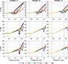 |
Figure 4 Sound insulation, expressed via the sound reduction index R, of (top) wall, (mid) glass, and (bottom) total surface for each sound source position S1–S6 and format L1–L3. Responses for sources S7–S11 are omitted due to their overlap with those of S1–S6. Gray dashed lines denote the typical building acoustics range (50 Hz–5 kHz). |
Finally, the average outdoor-based indoor magnitude and impulse responses were computed for each sound source format and indoor receiver in accordance with the methodology described in Section 3. The results are presented in Figure 5 for illustration purposes. As it can be seen, the presence of multiple peaks in the magnitude responses indicates the average sound transmission through the individual elements of the façade structure. Among the three source formats, the most pronounced peaks are observed for Format L1. In particular, the influence of the wall surface becomes evident primarily within the coincidence region (see Fig. 4), whereas outside this region, the contribution of the glass surface dominates the overall sound reduction. Finally, a smoother trend in the sound reduction indices is observed as the distance between the sound source format and the façade structure increases (from Format L1 to L3).
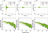 |
Figure 5 Average (top) impulse and (bottom) magnitude responses per indoor receive across all sound sources (S1–S11) in Format (left) L1, (mid) L2, and (right) L3. |
5.2 Experimental validation
For the validation of the modelling approach, the settings and the measurement results of the case study presented in [55] were used with respect to the distribution of three sound sources in a linear format in front of the façade of a rectangular-shaped classroom, representing a road-traffic structure scenario. An illustration of the characteristics of outdoor and indoor environments as well as building façade structures, including the measurement setup and equipment positions, is presentedin Figure 6.
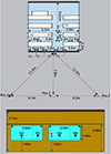 |
Figure 6 Schematic illustration of the experimental validation location and setup: (top) top-view of the indoor and outdoor environments, including the positions of sound sources (Pos.1–Pos.3) as well as of outdoor and indoor receivers (M1-M4), and (bottom) front-view of the building façade structure, including the positions of outdoor receivers. The centre of the façade in the top and front views is indicated by the purple and red markers, while the distances in the horizontal and vertical planes are denoted by the dashed black andblue lines. |
Regarding the façade structure from inside to outside, this consists of a plaster layer, a brick layer, a poroelastic layer and a metal layer with point connections. For simplicity, it was assumed that the façade structure consists of a three-layered structure composed by a brick (ρ = 1900 kg/m3, E = 2.4 ⋅ 1010 Pa, μ = 0.1, η = 0.01, and h = 0.050 m), a poroelastic (ϕ = 0.9, α ∞ = 1, σ = 59100 NS/m4, Λ = 10 μ Pa, Λ′ = 36 μ Pa, ρ = 90 kg/m3, E = 7 ⋅ 105 Pa, μ = 0.01, η = 0.01, and h = 0.070 m), and a steel surface (ρ = 7800 kg/m3, E = 2.1 ⋅ 1011 Pa, μ = 0.33, η = 0.01, and h = 0.026 m), assuming that the plaster layer does not significantly influence the sound reduction index. The windows consist of a double-layered structure, where the thickness of each layer is 5 mm and the gap between the two glass layers is 15 mm. The reverberation time of this room was obtained via the ISO 3382-2 [56]. The results of the averaged (over different source and outdoor-indoor receiver positions) measured and simulated sound insulation are presented in Figure 7.
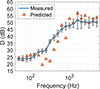 |
Figure 7 Comparison between the measured and calculated average sound insulation, expressed via the outdoor-indoor level difference (D) across the sound source and receiver positions in 1/3-octave frequency bands. The error-bars denote the 95% Confidence Interval. |
As shown in Figure 7, the predicted results closely follow the measured data, successfully capturing the main trends observed in the measurements. Deviations between predicted and measured levels can be attributed to uncertainties in the material properties of the façade layers, such as Young’s modulus and the damping loss factor. Additional discrepancies are likely influenced by characteristics of the incident acoustic field, as well as by factors not explicitly accounted for in the modelling framework, including the modal behaviour of structural surfaces, the influence of window frames, and their connections to the surrounding building elements. Furthermore, the measured weighted apparent sound reduction index (R w ′) of the façade is 42 dB, while the simulated value is 37 dB, resulting in a difference of 5 dB. This moderate discrepancy is within an acceptable range for predictive acoustic modelling, especially considering the modelling restrictions and the uncertainties described above. The single-valued results indicate that the simulation captures the primary acoustic behavior of the façade with satisfactory accuracy.
The degree of uncertainty observed at high frequencies, reflected by the confidence intervals in each 1/3-octave band, can be attributed to the positioning of the outdoor microphone receivers on the window surfaces, which are associated with the dominant transmission pathway, in relation to the façade design.
Additionally, the degree of uncertainty associated with the impact of the direct sound field on the averaged outdoor-to-indoor level differences in the experimental validation location (Fig. 6), was evaluated in [55]. In particular, the measurements were analyzed for the three sound source positions (Pos.1–Pos.3), the four outdoor receivers (M1–M4), and all indoor receivers. The analysis revealed that the relative positioning of the sound source and outdoor receiver has a significant influence on the level differences, as evidenced by the wide confidence intervals presented in Figure 7. Finally, the high degree of uncertainty may influence the evaluation of exposure-response relationships.
5.3 Relationship between indoor-outdoor noise levels
Outdoor and indoor noise level relationships based on the defined scenarios were explored with respect to the equivalent, maximum, and percentile noise indicator, including the time-averaged equivalent spectral outdoor-to-indoor level differences in the typical sound insulation range between 50 Hz and 5 kHz. However, for the sake of convenience, the results associated with Room 1 and Format L1, corresponding to the most prominent results, are presented and discussed here. A similar analysis can be undertaken with regard to the remaining two sound source formats, as well as those pertinent to the other two room scenarios.
Despite the fact that four façade structures are under consideration, only two of them are discussed. First, the relationship between indoor and outdoor levels for a double-leaf wall filled with mineral wool and a single-leaf window was studied with respect to the equivalent indicator. In addition, the time-averaged equivalent spectral outdoor-to-indoor level differences were also considered. Both results are presented in Figure 8.
 |
Figure 8 Relationship between average outdoor and indoor levels (left) across all receivers and sound sources in Format L1 for Room 1 with the façade structure composed of a single-leaf window and double-leaf wall surface, including the time-averaged equivalent spectral outdoor-to-indoor level differences (right). Note that “°"/“×" (levels per 15 s) and “—”/“- -" correspond to h w = 0.1m/0.2m. Values in the legend denote window thicknesses. |
As seen in Figure 8 (left), an increase in the window surface area results in a greater transmission of energy into the interior space, which is accompanied by a reduction in the outdoor-to-indoor level difference. For the smallest window size scenario, the impact of the wall surface is observed to prevail over that of the window surface, which is evident from the fact that the outdoor-to-indoor level differences are not related to the window thickness. Focusing on the average spectral characteristics of the outdoor-to-indoor levels in Figure 8 (right), two dips below 1 kHz are present in the lowest window size scenario, corresponding to the coincidence frequencies of the wall surfaces. The (first) coincidence frequency of the thicker wall structure exhibit a lower frequency dip than that of the thinner structure. In regard to the window surface, the coincidence frequencies occur at higher frequencies, particularly above 1 kHz. Furthermore, the mass-air-mass (resonance) frequencies of the (two) wall structures are situated at approximately 30 Hz and 20 Hz. Focusing on the largest in-size window structure, the single-leaf window structure dominates over the double-leaf wall structure, yielding comparable spectral characteristics to those observed in the single-leaf wall and window scenario.
Given the comparable outcomes observed in the double-leaf and triple-leaf window structures, only the impact of the double-leaf window on the double-leaf wall structure filled with mineral wool will be discussed here. The results are presented in Figure 9. As seen in Figure 9, analogous patterns to those depicted in Figure 8 are evident. Regarding the small-sized window, the indoor levels are found to be lower in comparison to those observed in the previous conditions. This is due to a slightly higher impact of the double window structure in comparison to the respective single window structure. In the case of the mid-sized window scenarios, there are scenarios that the mass-air-mass resonance frequencies of the windows overlap with the lowest coincidence frequencies of the wall surface. However, in the examination of the large-sized window structure, it becomes evident that an increase in the thickness of the leaves results in a shift towards lower frequencies in the mass-air-mass resonance frequency of the glazing surface. Finally, an increase in the cavity depth of window structures does not yield a significant difference in the small-sized window. The differences are evident in their (spectral) levels, particularly at higher frequencies. In scenarios involving mid-sized and large-sized windows, it has been observed that the lowest coincidence frequencies undergo a shift towards lower frequencies as the cavity size of the windows increases.
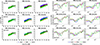 |
Figure 9 Relationship between average outdoor and indoor levels (left) across all receivers and sound sources in Format L1 for Room 1 with the façade structure composed of a double-leaf window and wall surface, including the time-averaged equivalent spectral outdoor-to-indoor level differences (right). Note that “°"/“×" (levels per 15 s) and “—"/“ - -" correspond to h w = 0.1m/0.2m, while d g denotes the window cavity width. Values in the legend denote window thicknesses. |
5.4 Prediction modelling
All tuned modelling approaches described in Section 4.3 were evaluated using the R2 and root mean square error (RMSE) metrics with respect to the training datasets. The results, presented in Table 4 for various noise indicators, show that the step-wise regression (SW) approach yielded the lowest performance (RMSE ≈ 2.8–2.9 dB). The highest accuracy was achieved by the random forest (RF) model (RMSE ≈ 1.0–1.3 dB), followed by the neural network (NN) model (RMSE ≈ 2.5–2.6 dB). The performance of the models was further validated using the test datasets, with results shown in Table 5. Consistently across all noise indicators, the random forest approach demonstrated the best performance (RMSE ≈ 1.5–1.7 dB), followed by the neural network model (RMSE ≈ 2.5–2.7 dB). The step-wise regression approach again showed the lowest accuracy (RMSE ≈ 2.8–2.9 dB).
Modelling diagnostics based on the training dataset.
Modelling diagnostics based on the test dataset.
The RMSE levels can be interpreted in the context of the human ear’s sensitivity to detect changes in broadband noise levels, corresponding to perceptible level differences. Specifically, RMSE levels of 3 dB and 5 dB are associated with just perceptible and clearly perceptible level differences, respectively [57]. Within this framework, all the modelling approaches yielded predictions with RMSE levels below the 3 dB threshold, indicating that the associated errors remain below the level of just noticeable level difference. In particular, RMSE levels for the random forest and neural network approaches were found to be substantially and moderately below the threshold for just perceptible level difference, respectively, whereas the step-wise regression approach yielded levels approaching this threshold.
Given the best performance of the random forest models, a comparison was conducted between the predicted and observed indoor noise levels using the test datasets, with RMSE levels detailed in Table 5. The results of this comparison are illustrated in Figure 10. As shown, the models demonstrate improved accuracy in estimating higher noise levels. In lower levels, increased deviations between predicted and observed levels are attributed to variations in the façade sound insulation characteristics.
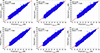 |
Figure 10 Validation of random-forest models for the L eq (top-left), L max (top-mid), L 01 (top-right), L 05 (bottom-left), L 10 (bottom-mid), and L 50 (bottom-right) noise indicators. Observed levels are derived from the computational model, while predicted levels are estimated using the random forest approach. |
The relative importance of each predictor in the estimation of indoor noise exposure levels was assessed through the application of Random Forest models, as depicted in Figure 11. As shown across all subplots, the highest normalized importance values were consistently attributed to the outdoor noise exposure levels, expressed via the noise indicators, indicating that the prediction of indoor sound pressure levels is primarily governed by outdoor levels rather than building (façade) or source characteristics. The window-to-façade area ratio (SRatio) was identified as a consistent second contributor in all models. Given that this parameter quantifies the proportion of the façade occupied by window elements, its influence underscores the role of glazing surfaces in outdoor-to-indoor sound transmission. The spatial distance between the building façade and the sound source format (FrmDist) was shown to be a consistent third contributor in all models, suggesting that the relative positioning of the sound source affects indoor noise levels. In all the models, construction-related features of the window structures, specifically glazing thickness (hGlass) and the width between glazing panes (dGlass), contributed more than those of the wall structures. These findings suggest that the acoustic insulation performance of the window system plays a more prominent role in mitigating indoor noise exposure compared to that of the wall structures. This trend is further supported by the moderate importance attributed to the window structural type (WinStruct). Conversely, minimal contributions were consistently observed for room volume (RoomVol), wall structure (WallStruct), and wall thickness (hWall) across all model configurations. Although these variables are acknowledged as relevant to indoor acoustic conditions, their relative influence was minor compared to predictors associated with window systems.
 |
Figure 11 Normalized importance per predictor with respect to the random-forest modelling approach for the L eq (top-left), L max (top-mid), L 01 (top-right), L 05 (bottom-left), L 10 (bottom-mid), and L 50 (bottom-right) indicator. |
Finally, to evaluate the relative importance of predictors in the predictive models, a systematic leave-one-variable-out procedure was conducted using the random forest approach with respect to the test dataset. Each predictor, except for the outdoor noise exposure levels expressed via the various noise indicators (equivalent, maximum, and percentile indicators), was individually removed from the models, and performance metrics (R2 and RMSE) were computed and compared to those of the full model, which included all predictors. This approach enabled the quantification of the marginal contribution of each variable to the overall predictive power. The analysis was repeated across all the noise indicator models, and the results are presented in Figure 12. As seen in Figure 12, the removal of the low-importance WallStruct predictor resulted in a minimal mean R2 drop of 0.09% (±0.02%) and an RMSE increase of 0.83% (±0.17%). Similarly, excluding the RoomVol and hWall predictors led to modest R2 reductions of 0.23% (±0.22%) and 0.50% (±0.06%), respectively, with corresponding RMSE level increases of 2.14% (±2.11%) and 4.47% (±0.49%). Moderate impacts were observed when WinStruct and dGlass predictors were removed, with mean R2 drops of 2.33% (±0.10%) and 6.04% (±0.55%), and RMSE increases of 19.32% (±1.57%) and 44.99% (±4.38%), respectively. The exclusion of hGlass and FrmtDist predictors produced more substantial effects, reducing R2 by 12.57% (±0.17%) and 12.61% (±0.18%) and increasing RMSE by 81.55% (±8.24%) and 81.83% (±8.24%). The most significant performance degradation occurred upon removal of SRatio predictor, which led to a mean R2 decline of 48.25% (±1.62%) and a pronounced RMSE increase of 213.28% (±21.65%). These results indicate a clear hierarchy of predictor importance, with a huge impact on predictive accuracy when the most influential variables are omitted.
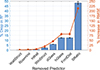 |
Figure 12 Percentage drop in R 2 (blue bars, left y-axis) and percentage increase in RMSE levels (orange line with markers, right y-axis) following the exclusion of individual predictors from the random forest model. Error bars represent standard deviations across the noise indicator models. Predictors are ordered by increasing impact on performance loss. |
6 Conclusions
In this work, a modelling framework for outdoor-to-indoor sound propagation was developed based on sound insulation principles. The framework integrates the Transfer Matrix Method (TMM), the spatial window technique, and bridge connection, allowing for the representation of multi-component façade structures, comprising wall, with single- to double-layered configurations, and window elements, with single to triple-layered configurations. This enables the synthesis of outdoor-based indoor impulse responses, which, when convolved with recorded signals (e.g., road traffic noise), support the estimation of indoor noise exposure levels using objective indicators such as equivalent, maximum, and percentile sound pressure levels. The method offers a controlled and reproducible approach to indoor sound exposure assessment. The integration of multi-layered, multi-component façades into the TMM framework enhances its applicability while preserving computational efficiency. As such, the proposed framework could well suited for applications in virtual acoustics, real-time auralization, and psychoacoustic research, particularly where low computational cost and high temporal resolution are critical.
A statistical learning framework was also developed to enable the investigation of exposure-response relationships between estimated indoor noise levels and health outcomes, utilizing either simulated data or hybrid datasets that combine simulations and measurements. In this study, synthesized datasets were generated based on the computational modelling framework, allowing for the evaluation and estimation of outdoor-to-indoor sound propagation through statistical learning approaches, with performance errors achieving levels below the just noticeable difference of 3 dB. Additionally, it facilitates the identification of key predictors associated with outdoor and indoor environments, as well as building façade structures. Using the developed framework, it was determined that outdoor noise exposure levels, along with factors related to window components and sound source position, constitute the most important predictors for estimating indoor noise exposure levels. This approach provides a more intuitive and comprehensive understanding of the ways in which environmental noise propagates from outdoors to indoors in built environments.
Funding
This research was funded by the European Union’s Horizon 2020 research and innovation program under grant agreement No. 874724, Equal-Life Project, part of the European Human Exposome network.
Conflicts of interest
The authors declare no conflict of interest.
Data availability statement
Data are available on request from the authors.
Author contribution statement
Michail Evangelos Terzakis: Conceptualization, Methodology, Software, Validation, Formal Analysis, Writing – Original Draft, Visualization. Cédric Van Hoorickx: Conceptualization, Methodology, Writing – Review & Editing, Supervision. Maarten Hornikx: Resources, Writing – review & Editing, Supervision, Project administration, Funding acquisition.
References
- S. Stansfeld, B. Berglund, C. Clark, I. Lopez-Barrio, P. Fischer, E. Öhrström, M.M. Haines, J. Head, S. Hygge, I. van Kamp, B.F. Berry: Aircraft and road traffic noise and children’s cognition and health: a cross-national study. The Lancet 365 (2005) 1942–1949. [CrossRef] [Google Scholar]
- I. van Kamp, H. Davies: Noise and health in vulnerable groups: a review. Noise and Health 15, 64 (2013) 153–159. [Google Scholar]
- I. van Kamp, S. Simon, H. Notley, C. Baliatsas, E. van Kempen: Evidence relating to environmental noise exposure and annoyance, sleep disturbance, cardio-vascular and metabolic health outcomes in the context of IGCB (N): a scoping review of new evidence. International Journal of Environmental Research and Public Health 17, 9 (2020) 3016. [Google Scholar]
- M.E. Terzakis, M. Dohmen, I. van Kamp, M. Hornikx: Noise indicators relating to non-auditory health effects in children – a systematic literature review. International Journal of Environmental Research and Public Health 19, 23 (2022) 15633. [Google Scholar]
- E. van Kempen, I. van Kamp, R.K. Stellato, I. Lopez-Barrio, M.M. Haines, M.E. Nilsson, C. Clark, D. Houthuijs, B. Brunekreef, B. Berglund, S.A. Stansfeld: children’s annoyance reactions to aircraft and road traffic noise. Journal of Acoustical Society of America 125, 2 (2009) 895–904. [Google Scholar]
- F. Minichilli, F. Gorini, E. Ascari, F. Bianchi, A. Coi, L. Fredianelli, G. Licitra, F. Manzoli, L. Mezzasalma, L. Cori: Annoyance judgment and measurements of environmental noise: a focus on Italian secondary schools. International Journal of Environmental Research and Public Health 15, 2 (2018) 208. [Google Scholar]
- M. Klatte, J. Spilski, J. Mayerl, U. Möhler, T. Lachmann, K. Bergström: Effects of aircraft noise on reading and quality of life in primary school children in Germany: results from the NORAH study. Environment and Behavior 49, 4 (2017) 390–424. [Google Scholar]
- P. Lercher, G.W. Evans, U. Widmann: The ecological context of soundscapes for children’s blood pressure. Journal of Acoustical Society of America 134, 1 (2013) 773–781. [Google Scholar]
- A. Enoksson Wallas, C. Eriksson, A.K. Edstedt Bonamy, O. Gruzieva, I. Kull, M. Ögren, A. Pyko, M. Sjöström, G. Pershagen: Traffic noise and other determinants of blood pressure in adolescence. International Journal of Hygiene and Environmental Health 222, 5 (2019) 824–830. [Google Scholar]
- W. Babisch, H. Neuhauser, M. Thamm, M. Seiwert: Blood pressure of 8-14 year old children in relation to traffic noise at home – Results of the German Environmental Survey for Children (GerES IV). Science of the Total Environment 407, 22 (2009) 5839–5843. [Google Scholar]
- S. Stansfeld, C. Clark: Health effects of noise exposure in children. Current Environment Health Report 2, 2 (2015) 171–178. [Google Scholar]
- J. Lu, J. Wu, Y. Chen: Indoor environment and brain health across the life course: a systematic review. Building and Environment 267 (2025) 112156. [Google Scholar]
- A. Santoni, J.L. Davy, P. Fausti, P. Bonfiglio: A review of the different approaches to predict the sound transmission loss of building partitions. Building Acoustics 27, 3 (2020) 253–279. [Google Scholar]
- L. Cremer: Theorie der Schalldämmung von Wänden bei schrägem Einfall. Akustische Zeitschrift 7, 3 (1942) 81–104. [Google Scholar]
- F.J. Fahy, P. Gardonio: Sound and structural vibration: radiation, transmission and response, 2nd edn., Elsevier, 2007. [Google Scholar]
- J.L. Davy: Predicting the sound insulation of single leaf walls: extension of Cremer’s model. Journal of Acoustical Society of America 126, 4 (2009) 1871. [Google Scholar]
- J.L. Davy: Predicting the sound insulation of walls. Building Acoustics 16 (2009) 1–20. [Google Scholar]
- J.L. Davy: The improvement of a simple theoretical model for the prediction of the sound insulation of double leaf walls. Journal of Acoustical Society of America 127, 2 (2010) 841–849. [Google Scholar]
- N. Atalla, F. Sgard: Finite element and boundary methods in structural acoustics and vibration. CRC Press, Boca Raton, Florida, 2015. [Google Scholar]
- R. Panneton, N. Atalla: Numerical prediction of sound transmission through finite multilayer systems with poroelastic materials. Journal of Acoustical Society of America 100, 1 (1996) 346–354. [Google Scholar]
- T.E. Vigran: Building acoustics, 2nd edn., CRC Press, 2019. [Google Scholar]
- J.F. Allard, N. Atalla: Propagation of sound in porous media: modelling sound absorbing materials, 2nd edn., Wiley-Blackwell, 2009. [Google Scholar]
- M. Villot, C. Guigou, L. Gagliardini: Predicting the acoustical radiation of finite size multi-layered structures by applying spatial windowing on infinite structures. Journal of Sound and Vibration 245, 3 (2001) 433–455. [Google Scholar]
- M. Villot, C. Guigou-Carter: Using spatial windowing to take the finite size of plane structures into account in sound transmission. In: NOVEM 2005 Conference, Biarritz, France, 2005. [Google Scholar]
- T.E. Vigran: Predicting the sound reduction index of finite size specimen by a simplified spatial windowing technique. Journal of Sound and Vibration 325, 3 (2009) 507–512. [Google Scholar]
- S. Ghinet, N. Atalla: Sound transmission loss of insulating complex structures. Canadian Acoustics 29, 3 (2001) 26–27. [Google Scholar]
- P. Bonfiglio, F. Pompoli, R. Lionti: A reduced-order integral formulation to account for the finite size effect of isotropic square panels using the transfer matrix method. Journal of the Acoustical Society of America 139, 4 (2016) 1773–1783. [Google Scholar]
- Y. Yu, C. Hopkins: Reduced order integration for the radiation efficiency of a rectangular plate. JASA Express Letters 1, 6 (2021) 062801. [Google Scholar]
- M.E. Terzakis, C. Van hoorickx, M. Hornikx: Spatial windowing for finite-size incident sound transmission coefficient of multi-component surfaces. INTER-NOISE and NOISE-CON Congress and Conference Proceedings 270, 9 (2024) 2900–2909. [Google Scholar]
- T.E. Vigran: Sound transmission in multilayered structures – introducing finite structural connections in the transfer matrix method. Applied Acoustics 71, 1 (2010) 39–44. [Google Scholar]
- T.E. Vigran: Sound insulation of double-leaf walls – allowing for studs of finite stiffness in a transfer matrix scheme. Applied Acoustics 71, 7 (2010) 616–621. [Google Scholar]
- A. Santoni, P. Bonfiglio, P. Fausti, N.Z. Martello: Sound insulation of heavyweight walls with linings and additional layers: numerical investigation. In: EuroNoise 2015, Maastricht, 2015, pp. 2537–2542. [Google Scholar]
- A. Santoni, P. Bonfiglio, J.L. Davy, P. Fausti, F. Pompoli, L. Pagnoncelli: Sound transmission loss of ETICS cladding systems considering the structure-borne transmission via the mechanical fixings: numerical prediction model and experimental evaluation. Applied Acoustics 122 (2017) 88–97. [Google Scholar]
- B. Locher, A. Piquerez, M. Habermacher, M. Ragettli, M. Röösli, M. Brink, C. Cajochen, D. Vienneau, M. Foraster, U. Müller, J. Wunderli: Differences between outdoor and indoor sound levels for open, tilted, and closed windows. International Journal of Environmental Research and Public Health 15 1 (2018) 149. [Google Scholar]
- F. Naim, D. Fecht, J. Gulliver: Assessment of residential exposure to aircraft, road traffic and railway noise in London: relationship of indoor and outdoor noise. In: Euronoise 2018, Crete, Greece, 2018, pp. 2905–2912. [Google Scholar]
- M.E. Terzakis, C. Van hoorickx, M. Hornikx, F. Naim, A.L. Hansell, J. Gulliver: Estimation of low frequency outdoor-to-indoor noise attenuation factors based on night-time noise exposure. In: 30th International Congress on Sound and Vibration (ICSV), Amsterdam, The Netherlands, 2024, pp. 1–8. [Google Scholar]
- WHO: Burden of disease from environmental noise: quantification of healthy life years lost in Europe. European Centre for Environmental Health and JRC, EU, 2011. [Google Scholar]
- S. Pirrera, E. De Valck, R. Cluydts: Nocturnal road traffic noise assessment and sleep research: The usefulness of different timeframes and in- and outdoor noise measurements. Applied Acoustics 72, 9 (2011)677–683. [Google Scholar]
- F. Scamoni, C. Scrosati: The facade sound insulation and its classification. In: Forum Acusticum, Kraków, Poland, 2014. [Google Scholar]
- I. Muhammad, A. Heimes, and M. Vorländer: Interactive real-time auralization of airborne sound insulation in buildings. Acta Acustica 5 (2021) 19. [Google Scholar]
- I. Muhammad, A. Heimes, M. Vorländer: Sound insulation auralization filters design for outdoor moving sources. In: Proceedings of the 23rd International Congress on Acoustics, Aachen, Germany, 2019, pp. 1721–1728. [Google Scholar]
- ISO: ISO 12354-3:2017, Building acoustics – estimation of acoustic performance of buildings from the performance of elements. Part 3: Airborne sound insulation against outdoor sound. International Organization for Standardization, 2017. [Google Scholar]
- J. Proakis, D. Manolakis: Chapter 10 – Design of digital filters. In: Digital Signal Processing, 4th edn., Pearson, pp 660–664, 2006. [Google Scholar]
- H. Felhi, H. Trabelsi, M. Taktak, M. Chaabane, M. Haddar: Effects of viscoelastic and porous materials on sound transmission of multilayer systems. Journal of Theoretical and Applied Mechanics 56, 4 (2018) 961. [Google Scholar]
- RStudio Team: RStudio: Integrated Development Environment for R. RStudio, PBC, Boston, MA, 2020. [Google Scholar]
- M. Kuhn: Building predictive models in R using the caret package. Journal of Statistical Software 28, 5 (2008) 1–26. [Google Scholar]
- G. James, D. Witten, T. Hastie, R. Tibshirani: An introduction to statistical learning with applications in R. Springer US, New York, 2021, pp. 203–205. [Google Scholar]
- M.N. Wright, A. Ziegler: ranger: a fast implementation of random forests for high dimensional data in C++ and R. Journal of Statistical Software 77, 1 (2017) 1–17. [Google Scholar]
- B. Boehmke, B. Greenwell: Hands-on machine learning with R. Chapman and Hall/CRC, 2019. [Google Scholar]
- Y. Rothacher, C. Strobl: Identifying informative predictor variables with random forests. Journal of Educational and Behavioral Statistics 49, 4 (2023) 595–629. [Google Scholar]
- B. Lantz: Machine learning with R, 2nd edn., Packt Publishing, 2015. [Google Scholar]
- A. Liaw, M. Wiener: Classification and regression by RandomForest. R News 2 (2022) 18–22. [Google Scholar]
- A. Gulli, S. Pal: Deep learning with Keras. Packt Publishing Ltd, 2017. [Google Scholar]
- M. Abadi, P. Barham, J. Chen, Z. Chen, A. Davis, J. Dean, M. Devin, S. Ghemawat, G. Irving, M. Isard, M. Kudlur, J. Levenberg, R. Monga, S. Moore, D. Murray, B. Steiner, P. Tucker, V. Vasudevan, P. Warden, M. Wicke, Y. Yu, X. Zheng: TensorFlow: a system for large-scale machine learning. In: 12th USENIX Symposium on Operating Systems Design and Implementation (OSDI 16), Savannah, GA, USA, 2–4 November, 2016, pp. 265–283. [Google Scholar]
- M.E. Terzakis, C. Van hoorickx, M. Hornikx: Characterization of façade sound insulation by impulse response measurements for various source position formats: a case study. INTER-NOISE and NOISE-CON Congress and Conference Proceedings 270, 9 (2024) 2910–2920. [Google Scholar]
- ISO: ISO 3382-2:2008 Acoustic – measurement of room acoustic parameters, part 2: reverberation time in ordinary rooms. International Organization for Standardization, 2008. [Google Scholar]
- E. Murphy, E.A. King: Principles of environmental noise. In: Environmental noise pollution, Elsevier, 2014, pp. 9–49. [Google Scholar]
Cite this article as: Terzakis M.E. Van hoorickx C. Hornikx M. 2025. An outdoor-to-indoor sound propagation modelling framework for evaluating noise exposure applications 9, 61. https://doi.org/10.1051/aacus/2025050.
All Tables
Window scenarios per room. L g and H g denote the length and height of window surfaces, respectively. Additionally, S g, S w, S f denote the surface area of the window, wall, and total façade structure, respectively.
All Figures
|
Figure 1 Discretization of a rectilinear surface (black shape outline) into isolated (blue shape outline) and adjacent (red shape outline) sub-surfaces. |
| In the text | |
|
Figure 2 Adjusted radiation efficiency of a rectilinear glazing surface, computed using the zeroth-order σ(0)(kp) (blue) and first-order σ(1)(kp) (red) adjusted radiation efficiency, along with the numerically integrated reference curve σ(kp) (black). The gray dashed lines represent the typical frequency range in building acoustics, spanning from 50 Hz to 5 kHz. |
| In the text | |
|
Figure 3 Example case scenario, including the outdoor environment (left) and the indoor environment (right). |
| In the text | |
|
Figure 4 Sound insulation, expressed via the sound reduction index R, of (top) wall, (mid) glass, and (bottom) total surface for each sound source position S1–S6 and format L1–L3. Responses for sources S7–S11 are omitted due to their overlap with those of S1–S6. Gray dashed lines denote the typical building acoustics range (50 Hz–5 kHz). |
| In the text | |
|
Figure 5 Average (top) impulse and (bottom) magnitude responses per indoor receive across all sound sources (S1–S11) in Format (left) L1, (mid) L2, and (right) L3. |
| In the text | |
|
Figure 6 Schematic illustration of the experimental validation location and setup: (top) top-view of the indoor and outdoor environments, including the positions of sound sources (Pos.1–Pos.3) as well as of outdoor and indoor receivers (M1-M4), and (bottom) front-view of the building façade structure, including the positions of outdoor receivers. The centre of the façade in the top and front views is indicated by the purple and red markers, while the distances in the horizontal and vertical planes are denoted by the dashed black andblue lines. |
| In the text | |
|
Figure 7 Comparison between the measured and calculated average sound insulation, expressed via the outdoor-indoor level difference (D) across the sound source and receiver positions in 1/3-octave frequency bands. The error-bars denote the 95% Confidence Interval. |
| In the text | |
|
Figure 8 Relationship between average outdoor and indoor levels (left) across all receivers and sound sources in Format L1 for Room 1 with the façade structure composed of a single-leaf window and double-leaf wall surface, including the time-averaged equivalent spectral outdoor-to-indoor level differences (right). Note that “°"/“×" (levels per 15 s) and “—”/“- -" correspond to h w = 0.1m/0.2m. Values in the legend denote window thicknesses. |
| In the text | |
|
Figure 9 Relationship between average outdoor and indoor levels (left) across all receivers and sound sources in Format L1 for Room 1 with the façade structure composed of a double-leaf window and wall surface, including the time-averaged equivalent spectral outdoor-to-indoor level differences (right). Note that “°"/“×" (levels per 15 s) and “—"/“ - -" correspond to h w = 0.1m/0.2m, while d g denotes the window cavity width. Values in the legend denote window thicknesses. |
| In the text | |
|
Figure 10 Validation of random-forest models for the L eq (top-left), L max (top-mid), L 01 (top-right), L 05 (bottom-left), L 10 (bottom-mid), and L 50 (bottom-right) noise indicators. Observed levels are derived from the computational model, while predicted levels are estimated using the random forest approach. |
| In the text | |
|
Figure 11 Normalized importance per predictor with respect to the random-forest modelling approach for the L eq (top-left), L max (top-mid), L 01 (top-right), L 05 (bottom-left), L 10 (bottom-mid), and L 50 (bottom-right) indicator. |
| In the text | |
|
Figure 12 Percentage drop in R 2 (blue bars, left y-axis) and percentage increase in RMSE levels (orange line with markers, right y-axis) following the exclusion of individual predictors from the random forest model. Error bars represent standard deviations across the noise indicator models. Predictors are ordered by increasing impact on performance loss. |
| In the text | |
Current usage metrics show cumulative count of Article Views (full-text article views including HTML views, PDF and ePub downloads, according to the available data) and Abstracts Views on Vision4Press platform.
Data correspond to usage on the plateform after 2015. The current usage metrics is available 48-96 hours after online publication and is updated daily on week days.
Initial download of the metrics may take a while.