| Issue |
Acta Acust.
Volume 10, 2026
|
|
|---|---|---|
| Article Number | 1 | |
| Number of page(s) | 13 | |
| Section | Audio Signal Processing and Transducers | |
| DOI | https://doi.org/10.1051/aacus/2025067 | |
| Published online | 07 January 2026 | |
Scientific Article
Achieving broadband directivity control with dual corona discharge transducers
Ecole Polytechnique Fédérale de Lausanne, Laboratory of Wave Engineering LWE, Lausanne, Switzerland
* Corresponding author: This email address is being protected from spambots. You need JavaScript enabled to view it.
Received:
20
August
2025
Accepted:
27
November
2025
Abstract
Loudspeakers inherit their directivity from their geometry and dimensions. Enclosed loudspeakers are omnidirectional in the low frequency range, but their directivity depends on frequency for wavelengths smaller than the radiator size, precluding the directional control over the whole bandwidth. Loudspeakers pairs allow achieving simultaneously monopolar (in-phase) and dipolar (out-of-phase) sources, thus allowing directivity control. However, they are limited by their bulkiness, preventing extending controllable directivities over high frequencies. The Corona Discharge transducer (CDT) concept relies on ionizing an ultra-thin layer of air and oscillating it through an alternating electric field, generating sound without resorting to a mechanical membrane. This transducer combines a monopolar source linked to heat exchanges, and a dipolar linked to electrostatic forces, although these two sources strengths are interconnected, yielding a given unidirectional directivity. In this paper, we propose to leverage the combination of monopole and dipole at the heart of the CDT concept to achieve controllable directivities by stacking two independent CDTs. The very thin dimensions of the CDT allows achieving coincident controllable monopolar and dipolar sound sources making the control of directivity over the whole operating frequency ranges. An analytical model of the dual CDTs concept is first compared to full-wave simulations, and an experimental prototype is finally assessed in anechoic conditions. Our findings open the way to a new range of broadband directionally-controllable transducers that have application to sound generation, active noise reduction, or even non-reciprocal active acoustic metamaterials.
Key words: Plasma loudspeakers / Corona discharge transducer / Directivity control
© The Author(s), Published by EDP Sciences, 2026
 This is an Open Access article distributed under the terms of the Creative Commons Attribution License (https://creativecommons.org/licenses/by/4.0), which permits unrestricted use, distribution, and reproduction in any medium, provided the original work is properly cited.
1 Introduction
The development of techniques aiming at controlling the directivity of electroacoustic transducers is conventionally driven by (spatial) audio motivations [1], such as improving sound coverage over a targeted zone [2, 3], spatially localizing sound sources [4, 5] or avoiding back reflections in sound reinforcement contexts [6]. Similar techniques are also deployed in active noise cancellation contexts, either to separate the upstream and downstream sound fields on the sensor’s side [7], or to directionally steer noise reduction performance on the actuator’s side [8–12]. Furthermore, controlling the directivity of sound sources is particularly timely in the context of active metasurfaces achieving anomalous refraction of sound [13, 14], active non-reciprocal metamaterials [15–17], and even at the heart of the Willis coupling which has attracted a significant attention in recent years [18–21]. Although all directivity control techniques generally apply to both sensors (microphones) and actuators (loudspeakers), the focus will be put on loudspeaker systems in the following.
Loudspeakers directivities are inherently dependent on frequency. Generally a loudspeaker system (driver + cabinet) is considered almost omnidirectional for wavelengths that are larger than the largest dimension of the loudspeaker system. But as frequency increases above the k dmax = 1 “diffraction limit” (where dmax is the largest dimension and k the wavenumber), diffraction enters into play and yields frequency (relative to size)-dependent directivity patterns, that are inherently uncontrollable (as fixed by design) [22]. That means a given construction inevitably yields a given directivity. Besides resorting to additional waveguides and horn radiators, likely to increase the loudspeaker systems dimensions [23], several techniques have been developed in a view to controlling the directivity of electroacoustic transducers, provided the wavelength of operation is larger than the individual transducer dimensions. The most widespread delay-and-sum beamforming (DSB) consists in feeding a line (or surface) array of N loudspeakers with time-delayed versions of a given audio signal in order to steer sound power towards a prescribed direction in space [23, 24]. By deploying sub-arrays, it is even possible to extend the bandwidth of operation, but still limited by the system dimensions [25]. Parametric arrays leverage ultrasound focusing, relying on tiny ultrasound speakers (the reduced size of which allows covering a rather large frequency bandwidth), mapping the audible range by modulating two ultrasound signals of slightly different frequencies [26]. Although performing in achieving highly directional sound beams, these techniques require a significant processing power. Therefore, much simpler directivity control configurations, such as gradient loudspeakers resorting to only a pair of sound sources, allow achieving unidirectional directivities [27] although still governed by the diffraction limit. The following will rely on the latter technique as a simple use-case of directivity control with Corona Discharge Transducers (CDTs).
The CDT reported in reference [28] consists of an ultra-thin layer of partially-ionized air particles that is put in motion within an intense, oscillating electric field, allowing moving the surrounding medium and generating sound without resorting to a physical mechanical radiator. This transduction principle is characterized by a combination of two sound sources: one monopolar source resulting from local heat release of the corona discharge, and one dipolar source linked to the back and forth electrostatic force. Although the two sources are interdependent (and proportional to the driving voltage, with fixed relative strengths), the very thin dimension of the CDT makes them almost coincident, making this type of loudspeaker an almost frequency-independent unidirectional sound source along the axis normal to the radiating surface (however, its lateral geometry and dimensions inevitably yield a prescribed directivity). We will show in the following how stacking two adjacent CDTs fed with different input voltages allows independently controlling the monopolar and dipolar sources. The latter configuration then allows achieving interesting directivity patterns, still outperforming conventional loudspeakers owing to their very thinness.
This paper reports a concept of dual CDTs achieving controllable unidirectional patterns over a broad frequency range. In a first section, the fundamental principle of the CDT is reminded, followed by the formulation of the sound field generated by a dual CDTs. Then, numerical simulations are provided, which are finally experimentally verified on a laboratory prototype. Concluding remarks lead to discussion on the applicability of the dual CDTs to directional audio, as well as active noise control [29] and as a unit-cell for active metamaterials and metasurfaces [30].
2 The corona discharge transducer
2.1 Description of the transduction principle
Corona discharge transducers (CDTs) allow for sound generation thanks to the ionization of molecules in the surrounding fluid, moved by an intense oscillating electric field. In the “wire-to-grid” configuration, the transducer is constituted by a pair of electrodes (forming two parallel planes, as illustrated in the sketch of Fig. 1): the first one is a perforated metallic grid electrically connected to the ground, and is designated the “collector electrode”; the second one, designated “corona electrode”, is made of an ultra thin wire (diameter of the order of 100 μm), arranged in a pattern of parallel lines along a same plane parallel and distant of d to the collector plane, put at a sufficiently high voltage so as to trigger the extraction of electrons from surrounding molecules. The breakdown voltage U0, above which ionization occurs, depends on the geometry of the CDT (inter-electrode distance, corona wires diameter) and on the medium properties (relative permittivity, density, temperature, etc.), and is of the order of a few kVs in our study. As an order of magnitude, for a square CDT with a width in the range of 100 mm, a corona wire diameter of 0.1 mm, a distance between two consecutive corona wires in the range of 10 mm, and the gap between the collector and the corona wires in the range of 5 mm, the breakdown voltage in the air is in the range of 6 kV.
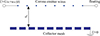 |
Figure 1. Schematic cut view of the electrode pair: the corona electrode consisting of an array of ultra-thin emitter wires parallel to each others (thin dots in this cut view), and a collector electrode consisting of a grounded perforated grid (dashed thick line in this cut view). |
When applying an offset voltage UDC higher than U0, the positive ions are accelerated from the ionization region (a few μm around the corona wires) towards the collector electrode. They then collide with the neutral particles present in the drift region (the inter-electrode space), which are then moved, giving rise to an “ionic wind” (constant flow). If an alternating voltage uac(t) is superimposed to UDC (ensuring total voltage UDC + uac remains higher than the breakdown voltage), the transducer makes the surrounding fluid medium oscillate, responsible for sound generation.
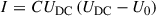
The preceding studies [28, 31, 32] have shown that this corona discharge transducer configuration could be modeled as a combination of two volumetric sound sources, one monopolar “heat” source H (due to the heat release around the corona electrodes), and another dipolar “force” source F (relative to the electrostatic force moving the surrounding fluid back and forth), the orientation of which depends on the sign of the ac voltage: a positive uac yields a force oriented towards the collector electrode and vice-versa.
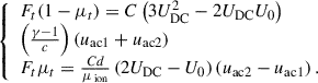
An extremely simple electroacoustic model can be deduced from the coupling equations between the plasma generation, and the two sound sources strengths. Indeed, it has been shown that the offset voltage UDC can be linked to the current I flowing through the corona wire according to the Townsend formula [32, 33]:
 (1)
(1)
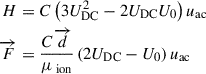
where C is a constant that depends on the transducer geometry, and that can be experimentally determined. Note that equation (1) still holds for oscillating voltages, when substituting UDC + uac for UDC. It is then possible to express the two sources strengths H and F as a function of the voltage feeding the transducer [28, 30, 32]. Assuming the ac voltage is much lower than the DC one, it is possible to linearize the expression of equation (1) and express linear relationships between the heat source power H (in W) and bulk electrostatic force F (in N) as:
 (2)
(2)
where μion designates the mobility of the ions, and  is the vector orthogonal to the electrode planes, defined from the corona electrode to the collector electrode (
 the plasma thickness).
It can be observed that the two sound sources are interdependent. Their individual influence is independent on frequency but on the constant parameters U0, UDC, C, d and μion, and indirectly on the transducer cross-section area S. Also, the lateral dimensions of the CDT are likely to change the current-voltage law (Eq. (1)), thus C.
For the numerical study of Section 4, we will define the heat source power density 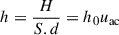 (in W/m3), and the dipolar force source density
 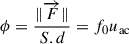 (in N/m3), where S is the transducer effective cross-section area.
2.2 Sound field generated by a single CDT
Let’s consider a square CDT of cross-section area S = w
2 where w is the square width, and thickness d (here the square geometry has been chosen for simplifying the fabrication of the prototype, but the following could also apply to any shape, for example a circular one). The corona electrode is made of a pattern of parallel thin wires (colored in deep purple), while the collector electrode is made of a perforated grid, illustrated with the black dots pattern. We will consider a spherical coordinates system ( ), whose origin O is located at the CDT geometrical center, as illustrated in Figure 2. In this system,
  is the distance to center O, angle θ designates the elevation with respect to z, and angle φ designates the azimuth over the CDT reference plane (parallel to the electrodes planes comprising O). In addition to this coordinates system, we will denote z the axis normal to the CDT reference plane, with unit vector
  . In this orientation, we can notice that
  , thus a negative sign in the following expressions of the electrostatic force. We will assume d ≪ λ where λ denotes the wavelength, yielding the two sources centers (heat and force sources) are collocated at O. As d is of the order of 5 mm, this assumption holds up to 10 kHz. In this example, the height of the corona electrode is supposed much smaller than the lateral dimension w of the transducer: d ≪ w ≪ λ.
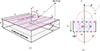 |
Figure 2. Sketch of a square CDT in free field: (a) 3D representation with cartesian and spherical coordinates definitions; (b) simplified cut view in the x O z plane. The blue circle represents the monopolar heat source, while the red circle pair highlights the dipolar force source, and their relative strength being qualitatively represented by the circles radii. |
We can then derive the wave equation as [28]:
 (3)
(3)
where γ is the specific heat ratio (equal to 1.4 in the air in adiabatic transformation). This can be formulated in the frequency domain as:
 (4)
(4)
where k is the wavenumber.
In case where the heat and force sources were considered as point sources and collocated (same position  ), the integration of equation (4) using the Green’s function
  would result in [22, 31, 32]:
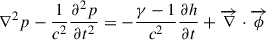
![Mathematical equation: $$ \begin{aligned} p(\overrightarrow{r})&=\int \int \int _V\left[-j\omega \dfrac{\gamma -1}{c^2}h + \overrightarrow{\nabla } . \overrightarrow{\phi } \right] g\left(\overrightarrow{r}|\overrightarrow{r_0}\right)\,\mathrm{d}V_0\nonumber \\&= jk\left[\dfrac{\gamma -1}{c} \underbrace{\int \int \int _V h \,\mathrm{d}V_0}_{H} + {\text{ sgn}}\left(\overrightarrow{d} \cdot \overrightarrow{e}_z\right)\left(\dfrac{j}{kr}+1\right)\right.\nonumber \\&\quad \times \left. \cos {\theta } \underbrace{\int \int \int _V \phi \,\mathrm{d}V_0}_{F=||\overrightarrow{F} ||} \right]\dfrac{e^{-jkr}}{4\pi r} \end{aligned} $$](/articles/aacus/full_html/2026/01/aacus250124/aacus250124-eq15.gif) (5)
(5)
where the sign of the force source depends on the orientation of the electrode pair with respect to the axis z, and H and  are derived by linearization and expressed in equation (2). As the ratio between H and F is assumed constant for a given transducer and given DC voltage UDC, the individual contributions of the heat and force sources on the total sound pressure, thus directivity DCDT(θ) resulting the heat and force point sources pair, are fixed by construction.
However, in the present case, the spatial extent of the sources is far from a point, and one needs to account for the directivity of the corresponding radiating surface. If we consider the radiation in the far field, the total radiated pressure can be derived as the product of the expression of equation (5) and the “geometric” directivity Dpiston(θ, φ) of the uniform piston of surface S.
In the case of a square piston of width w, the “geometric” directivity function reads [22]:
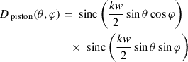 (6)
(6)
where sinc designates the sine cardinal function. We will intentionally disregard the radiation contribution of the small piston of cross-section area S to focus only on the heat and force source contributions DCDT(θ) to the overall directivity. However, one should bear in mind that the directivities will be affected by the geometry of the radiating square piston at high frequencies, as soon as  .
.
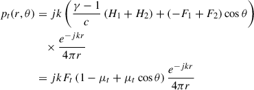
Let’s assume now that the transducer dimensions are much smaller than the distance of observation (r ≫ w ≫ d), so that the problem can be simplified as the one of point sources in a free spherical domain. Also, discarding the directivity of the piston, we can simplify the problem to a 2D axisymmetric problem, so that the spherical coordinates can be limited to only r and θ (φ may only appear in Dpiston(θ, φ)).
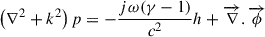
In the far field (k r ≫ 1), the sound pressure can be approximated as:
![Mathematical equation: $$ \begin{aligned} p(r,\theta ) = jk\dfrac{e^{-jk r}}{4\pi r} \underbrace{ \left[ \dfrac{(\gamma -1)}{c} {H} - {F}\cos \theta \right]}_{{F_{\text{ CDT}}}}. \end{aligned} $$](/articles/aacus/full_html/2026/01/aacus250124/aacus250124-eq19.gif) (7)
(7)
The term inside the brackets of equation (7) corresponds to the pressure forces exerted by the combination of the monopolar and dipolar sources at any angles θ over the boundaries of the dual CDTs, that can be rewritten to take the form of a unidirectional function:
![Mathematical equation: $$ \begin{aligned} \begin{aligned} {F_{\text{ CDT}}}(\theta )&= {F_t} \underbrace{\left[(1-\mu ) +\mu \cos (\theta +\pi )\right]}_{D_{\text{ CDT}}(\theta ) - \text{ unidirectional}} \end{aligned} \end{aligned} $$](/articles/aacus/full_html/2026/01/aacus250124/aacus250124-eq20.gif) (8)
(8)
where 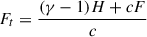 is a total force (in N, independent on frequency) and
 ![Mathematical equation: $ \mu=\frac{cF}{(\gamma-1)H+cF} \in [0,1] $](/articles/aacus/full_html/2026/01/aacus250124/aacus250124-eq22.gif) (dimensionless, independent on frequency) is the ratio of the bidirectional source to the overall directivity.
(dimensionless, independent on frequency) is the ratio of the bidirectional source to the overall directivity.
Then, with one single CDT, it is possible to achieve a given directivity DCDT(θ), prescribed by the ratio between the Heat “weight” (1 − μ) and the Force “weight” (μ), for any frequency. The following section will show how to decouple the monopole and dipole sources, and then fully control the directivity when two CDTs are stacked back-to-back.
3 The dual corona discharge transducer
3.1 General description
Now we stack two CDTs with same shape and dimensions back-to-back, namely sharing a common collector electrode, as illustrated in Figure 3. For the sake of generality, we can consider that the two CDTs may present slight differences in terms of construction, thus giving rise to different electroacoustic parameters such as their coupling factors (C1 and C2), offset voltages (UDC1 and UDC2) or even breakdown voltages (U01 and U02). If they are individually driven by two different voltages uac1 and uac2, it will yield two different sets of monopolar sources (H1, H2) and dipolar sources (F1, F2). As in the preceding section, we will consider that the CDTs’ thicknesses are still much smaller than the wavelength of interest (for example if d = 5 mm, the total thickness is 1 cm, thus subwavelength up to the range of 5 kHz). Then, following the same assumptions as in Section 2.2, the total sound pressure in the far field becomes:
 |
Figure 3. Simplified sketch of a dual Corona Discharge Transducer – cut view along the x O z plane. The observation point is assumed in the far field (r1 ≈ r2 ≈ r ≫ d) where r1 and r2 are the distance to the centers of each individual CDT and r denotes the distance to the center of the dual CDTs. |
![Mathematical equation: $$ \begin{aligned} p_t(r,\theta )&= jk \left[ \left(\dfrac{\gamma -1}{c}H_1 - F_1 \cos \theta \right) \dfrac{e^{-jkr_1}}{4\pi r_1}\right.\nonumber \\&\quad +\left. \left(\dfrac{\gamma -1}{c} {H_2} + {F_2} \cos \theta \right) \dfrac{e^{-jkr_2}}{4\pi r_2}\right] \end{aligned} $$](/articles/aacus/full_html/2026/01/aacus250124/aacus250124-eq23.gif) (9)
(9)
where  and
and  are the distances of observations relative to the centers of each CDT
  and
and  . Without loss of generality, we can observe that the distance d between the two centers is much smaller than the distance of observation
 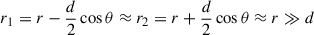 (see Fig. 3) and then:
 (10)
(10)
where 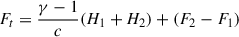 is a global force and
 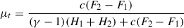 is the unidirectional factor of the dual CDTs arrangement, that both depend on uac1 and uac2 (and the parameters of the heat and force sources U
D
c
i
, U0i
, C
i
).
is the unidirectional factor of the dual CDTs arrangement, that both depend on uac1 and uac2 (and the parameters of the heat and force sources U
D
c
i
, U0i
, C
i
).
In the following, the directivity resulting from the monopole/dipole pair of the dual CDTs (discarding Dpiston) will be denoted:
 (11)
(11)
3.2 Case of ideally identical CDTs
In the ideal case where both CDTs share exactly the same physical properties, then feeding each with a same ac voltage uac1 = uac2 will cancel the dipolar terms (as the symmetry of the transducer yields opposite electrostatic force orientation on both sides of the collector electrode), thus achieving a fully monopolar source of amplitude  with H = H1 = H2:
 (12)
(12)
On the other hand, if the two CDTs are fed with opposite ac voltages (uac1 = −uac2), this will cancel the monopolar contributions and thus yields a fully bi-directional source of amplitude 2F with F = F2 = −F1:
 (13)
(13)
Finally, it is always possible to identify a combination of voltages uac1 and uac2 that allows achieving a targeted force F t and directivity D t (θ)=(1 − μ t )+μ t cosθ after:
 (14)
(14)
By denoting 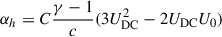 and
and 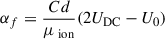 , the two sources coefficients, it finally yields:
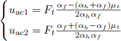 (15)
(15)
thus uac1 and uac2 can be directly derived from the settings of F t and μ t and vice-versa. A more practical protocol consists in setting one voltage (e.g. uac1) and prescribing a target unidirectional factor μ t , then it yields:
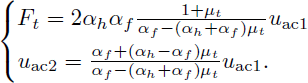 (16)
(16)
3.3 Case of CDTs with different characteristics
In the most general case where the electroacoustic properties of the two CDTs are unknown, or if they happen to present slight geometrical and electrical differences, we can generalize the preceding protocol to derive the voltages uac1 and uac2 allowing achieving a targeted directivity D t (θ) (and specifying for example one of the two ac voltages uaci ).
Let’s consider the two CDTs (denoted with subscript i) characterized by the following parameters:
-
offset voltage UDCi ;
-
breakdown voltage U0i ;
-
cross section area S i (affecting the current-voltage constant C i );
-
inter-electrode gap d i (affecting the current-voltage constant C i ).
In this case, the heat and force sources coefficients read:
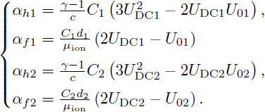 (17)
(17)
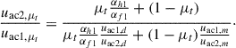
There exist pairs of voltages (uac1, m , uac2, m ) for which the dual CDTs arrangement yields an omnidirectional sound source (μ t = 0), and another pair (uac1, d , uac2, d ) for which the dual CDTs yields a bi-directional source (μ t = 1). Experimentally, it is possible to identify such two pairs of voltages (see Sect. 5.1) and deduce the relationships between α f1 and α f2 on the one hand, and between α h1 and α h2 on the other hand:
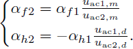 (18)
(18)
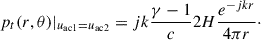
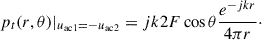
Also, computing the ratio between the sound pressures measured at a same distance r and at angle θ = 0 rad, for both cases (p m (r, 0)=p t (r, 0)| μ t = 0 for the monopole setting and p d (r, 0)=p t (r, 0)| μ t = 1 for the dipole setting), yields the ratio between α h1 and α f1 as:
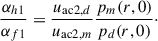 (19)
(19)
Parameters for the COMSOL model.
This ratio can finally be used to extract the voltage pair (uac1, μ t , uac2, μ t ) achieving the target directivity μ t after equation (14):
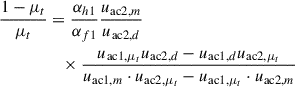 (20)
(20)
which finally yields:
 (21)
(21)
Note that this result shows a constant ratio between the two voltages feeding the dual CDTs, independent of frequency. Indeed, unidirectional factor μ
t
is a real gain ranging from 0 to 1, coefficients α
h
i
and α
f
i
are the real, frequency-independent, electroacoustic factors for the heat and force sources within each CDT i (similarly to the force factor for an electrodynamic transducer), and ratios  and
and  don’t depend on frequency neither. Then, the voltage ratio expressed in equation (21) represents a real gain between the two input voltages feeding the dual CDTs in a view to achieving a target directivity, independent of frequency, applying to any kind of signal, including audio signals.
In practice, we can fix one of the two CDT voltages (for example uac1) and keep the same value for all settings, in this case, uac1, m = uac1, d = uac1, μ t = uac1, ref, to simply derive uac2, μ t .
In the following, we will illustrate some examples of directivities achievable with the dual CDTs assembly.
4 Numerical simulations
In this section, we will give some examples of directivities simulated with COMSOL Multiphysics on a dual CDTs arrangement, as described in Section 3. In these simulation examples, we will consider two ideally identical CDTs, with constitutive parameters of Table 1, and follow the methodology described in Section 3.2. Note that the electrical parameters (C, U0, UDC) provided in this table are estimated beforehand by measuring the voltage-current curve on a prototype of same dimensions and geometry (here the square transducer prototype presented in Sect. 5). The interested readers can gain more insight on this calibration procedure in reference [32], page 49 and following.
4.1 Model geometry
The numerical model is designed using COMSOL Multiphysics Acoustic Module in 3D space dimension. The fluid domain is defined as a sphere of radius R = 3 m, with a Perfectly Matched Layer (PML) of 2 m, making the simulation extent of 5 m. Each of the individual CDT is modeled as identical parallelepipeds (Blocks) of square cross-section on the x
O
y plane, with width w and height d, sharing a common boundary at z = 0. We assume here the φ = 0 (x
O
z) and  (y
O
z), as well as the
(y
O
z), as well as the  planes, are symmetry planes, therefore simplifying the 3D domain comprised between planes φ = 0 and
  . This space domain simplification is highlighted in Figure 4a as a deep purple triangular surface over the reference plane z = 0 (corresponding to the shared collector electrode). The corresponding simplified COMSOL 3D model is illustrated on Figure 4b.
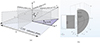 |
Figure 4. Model geometry in COMSOL Multiphysics: (a) Sketch of the dual CDTs reference plane (z = 0) highlighting symmetries, and definition of spherical coordinates angles θ and φ; (b) snapshot of the COMSOL 3D model simplified geometry. |
4.2 Model physics
The propagating domain, including the CDTs volume, is considered filled with air with mass density ρ and speed of sound c. Each CDT is modeled as the combination of a “Heat Source” of individual power density Qheat, i
= h0
uaci
where h0 is defined in Section 2.1 (also specifying the ratio of specific heat capacities γ and heat capacity at constant pressure C
P
), and a “Dipolar Domain Source” of individual volumetric force  , where i ∈ {1, 2} designates the CDT number 1 or 2 (as in Fig. 4). In this definition, the electrodes of the upper transducer CDT1 (resp. lower transducer CDT2) are arranged so that the projection of the electrostatic force
  (resp.
  ) over z is negative (resp. positive) for a positive uac1 (resp. uac2), as in the geometry presented in Section 3.
4.3 Other settings and processing methodology
The effect of the CDTs shape and dimensions on directivity start to enter into play for  where w = 13 cm, yielding a diffraction limit of approximately f
d
= 1 kHz. The study is performed in the frequency domain, for octave band frequencies spanning from fmin = 125 Hz to fmax = 1 kHz. The mesh inside the propagating domain and the CDTs is “Free Triangular” with maximal mesh size
where w = 13 cm, yielding a diffraction limit of approximately f
d
= 1 kHz. The study is performed in the frequency domain, for octave band frequencies spanning from fmin = 125 Hz to fmax = 1 kHz. The mesh inside the propagating domain and the CDTs is “Free Triangular” with maximal mesh size  , and the PML layer is meshed with a “Swept” mesh of maximum element size 10 cm.
The processing starts by specifying voltage uac1 as well as the target directivity parameter μ
t
. From these values, uac2 is set after equation (16), depending on the coefficients  and
and  . The results are presented in the following subsection.
4.4 Numerical results
4.4.1 Directivity
Figure 5 show the achieved directivities, along the plane  for different parameter settings μ
t
∈ {0, 0.3, 0.5, 0.63, 0.75, 1}. The first series of curves (plain lines) represent the directivities per octave band computed as the sound pressure magnitude over the boundary of the propagating medium (i.e. the interior boundary of the PML) divided by the maximum of sound pressure magnitude over this boundary:
for different parameter settings μ
t
∈ {0, 0.3, 0.5, 0.63, 0.75, 1}. The first series of curves (plain lines) represent the directivities per octave band computed as the sound pressure magnitude over the boundary of the propagating medium (i.e. the interior boundary of the PML) divided by the maximum of sound pressure magnitude over this boundary:
 |
Figure 5. Computed directivity |


![Mathematical equation: $$ \begin{aligned} D_{\text{ COMSOL}}(\theta )&=\frac{\left|p\left(r=R,\theta ,\varphi =\pi /4\right)\right|}{\max _{\theta \in [0,\pi ]}\left(\left|p\left(r=R,\theta , \varphi =\pi /4\right)\right|\right)},\nonumber \\&\quad \text{ for} \theta \in [0,\pi ]. \end{aligned} $$](/articles/aacus/full_html/2026/01/aacus250124/aacus250124-eq61.gif) (22)
(22)
The second series (plus markers) represents the same quantity defined from the theoretical value D t (θ) as in equation (11), multiplied by the square piston directivity Dsquare(θ, φ) of equation (6).
We can observe that the dual CDTs arrangement allows achieving the targeted directivites in each case (COMSOL and theoretical pressure fields perfectly match for each settings and each frequency). Also, we can see a deviation from the targeted directivity D
t
(θ) of equation (11) for frequencies f > 500 Hz, highlighting the directional characteristics of the square piston. This is particularly obvious for the omnidirectional directivity, where DCOMSOL(π/2)|500 Hz = 0.957 and DCOMSOL(π/2)|1000 Hz = 0.780. However, it can still be considered omnidirectional (for this specific case) up to 1 kHz as those directivity minima always exceed  .
.
4.4.2 Pressure along z axis
To further confirm the validity of the analytical model of the dual CDTs arrangement, the pressure as a function of distance along the z axis is also computed. The real and imaginary parts of the total sound pressure computed with COMSOL over the z axis at each frequency is then compared to the theoretical expression given in equation (10), also multiplied by the piston directivity of equation (6). The results obtained at f = 1 kHz are illustrated on Figure 6 for all cases. Although the far field condition is not fulfilled in the close vicinity of the dual CDT (distances shorter than λmin = 34 cm), we observe a good agreement between the COMSOL full wave simulations and the simple theoretical model elaborated in Section 3.2 in the far field (kr ≫ 1), validating the analytical model.
 |
Figure 6. Sound pressure (plain lines: real part; dashed lines: imaginary part) computed along the z axis with COMSOL Multiphysics (blue) and compared with the theoretical formulation of equation (10) at f = 1 kHz and for different values of μ t : (a) omnidirectional (μ t = 0); (b) subcardioid (μ t = 0.3); (c) cardioid (μ t = 0.5); (d) supercardioid (m u t = 0.63); (e) hypercardioid (μ t = 0.75); (f) bidirectional (μ t = 1). |
The next section will present experimental results obtained on a square dual CDTs prototype.
5 Experimental validation
The square dual CDTs is assembled on a common frame, constructed through additive manufacturing. A perforated grid made of Aluminium of thickness t = 1 mm is assembled in the median plane of the frame, and two networks of thin Tungsten wires of diameter dwire = 100 μm with inter-wire distance of 11 mm are assembled symmetrically on both sides, at a distance d = 5 mm to the metallic grid. The dual CDTs transducer is fed with DC+ac voltages from a custom dual-channel, High Voltage valve-based power amplifier, described in reference [32]. Figure 7 shows the construction principle and a picture of the experimental prototype taken from both sides.
 |
Figure 7. Dual CDT prototype. (a) Construction principle. (b) Front view. (c) Rear view. |
The dual CDTs is mounted on a microphone stand fixed to a Bruel & Kjaer Type 9640 Turntable System, and a PCB 378B02 half-inch microphone is aligned at 1 m from the dual CDTs center. The signal acquisition and processing is performed with a Bruel & Kjaer Type 3160 Pulse Multichannel Sound and Vibration Analyzer, each CDT channel on the power amplifier being excited with a synchronous swept sine ranging from 60 Hz to 2060 Hz with a sweep speed of 10 mdec/s, and individual voltages uac1 and uac2. The analysis consists in processing the transfer functions between the sound pressure sensed by the microphone and the output signal uac1 delivered to CDT1 amplification channel (that we set to a fixed value for all directivities). Figure 8 illustrates the experimental setup (the power amplifier and cabling are not visible here).
 |
Figure 8. Experimental setup. |
In this experimental evaluation, we will consider unknown CDTs parameters, following the methodology of Section 3.3.
5.1 Calibrating the directional corona discharge loudspeaker: Omnidirectional and bidirectional directivities
The first step consists in identifying the combination of voltages (uac1, m , uac2, m ) that gives rise to a pure omnidirectional directivity, and the pair (uac1, d , uac2, d ) that gives rise to a pure bidirectional directivity. To ensure the target directivity is achieved, two measurements of frequency responses are made for each settings:
-
Measurement at angles θ = 0 and
 for the omnidirectional target, and identification of the value for which both curves are optimally aligned.
 -
Minimization of the frequency response at angle
 for the bi-directional target.
Once the two voltage pairs are identified, the frequency responses (FRF) are measured for each angle  with integer n ∈ [0 : 36]. The measured FRFs for the omnidirectional setting are illustrated in Figure 9a every
  and for the bidirectional setting they are shown in Figure 9b every
  . We can observe that the frequency responses for both cases present the same high-pass behavior of 6 dB per octave, and that the response measured at θ = 0[π] rad in the bidirectional setting is about 12 dB higher than for the monopole setting, corresponding to the ratio of force to heat strengths
  . We can also note a glitch occurring in the measurements around 250 Hz, more prominent when signal to noise ratio is low (for example in the bidirectional setting, at angles around
  ), that might be the consequence of a notch filter effect due to a reflection on the metallic frame of the anechoic room (although the facility should be immune to such reflections).
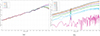 |
Figure 9. Frequency responses |
The corresponding directivity sampled at each octave central frequencies are illustrated in Figures 10a and 10f. The results reflect the calibration procedure, which allows determining the reference voltages pairs (uac1, m
, uac2, m
) and (uac1, d
, uac2, d
). The relative good agreement with the theoretical directivities (black plus markers) demonstrates the validity of the procedure up to 1 kHz. We can observe a slight misalignment at θ = 0[π] rad compared to the sensitivity at  for f = 125 Hz and 500 Hz in the omnidirectional setting (Fig. 10a), but the mismatch represents around 0.5 dB which can be considered satisfactory.
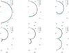 |
Figure 10. Directivity measured at different angles for: (a): omnidirectional (μ t = 0); (b) subcardioid (μ t = 0.3); (c) cardioid (μ t = 0.5); (d) supercardioid (μ t = 0.63); (e) hypercardioid (μ t = 0.75) and (f) bidirectional (μ t = 1) settings. For each case, the theoretical directivity D t (θ)=1 − μ t + μ t cosθ is presented with black plus markers. |
5.2 Achieving unidirectional directivities
Once the voltages pairs corresponding to μ t = 0 and μ t = 1 have been identified, the other pairs have been derived corresponding to any of the targeted μ t , following the methodology detailed in Section 3.3. The directivities achieved with the corresponding pairs of voltages (uac1, μ t , uac2, μ t ) for μ t ∈ {0; 0.3; 0.5; 0.63; 0.75; 1} are illustrated on Figure 10. Although some slight discrepancies might appear in the rear direction at certain frequencies for all of the measured unidirectional directivities, we can see a good agreement between the achieved directivities and the theoretical ones. These differences are mostly due to the rather short distance of measurement at 125 Hz and to the directivity of the square radiator at higher frequencies.
6 Conclusion
The control over directivity on conventional loudspeakers is known to be limited to low-frequencies due to their bulkiness. Given the compactness of the CDTs, it is possible to achieve very precise directivities in theory up to the range of 1 kHz following the proposed dual CDTs concept. In practice, however, the dimensions of the radiator induce a frequency limit above which the impact of planar geometry enters into play. But, in terms of directivity control, our results show that the introduced mechanism remains an advantageous asset, at least up to that frequency threshold, significantly outperforming loudspeakers of equal surface in realizing the targeted directivities. Though, it remains noticeably less performing in terms of overall sound power compared to conventional loudspeakers of same sizes, with a lower overall sensitivity and the typical high-pass behavior of its frequency response. This can be overcome by augmenting the radiating surface (though impacting the directivity performance), or further optimizing the electrodes arrangement (thinner corona wires, smaller air gap, etc.).
The dual CDTs concept has direct applications to directivity control on loudspeakers, owing to its direct conversion of electric voltage to acoustic flow velocity through the (geometry-dependent) radiation impedance. Besides, the dual CDTs will be an important asset as secondary source in ducted (1D) active noise reduction systems (e.g. active exhaust noise reduction). Indeed the capability to separate the net sound sources on each sides allows for controlling independently the up- and down-stream of the active control source, and thus have a full control over both sound fields individually. By extension, the dual CDTs will have direct application to active acoustic metamaterials and metasurfaces, as the control of monopolar/dipolar elements is at the heart of non-reciprocal concepts such as the Willis coupling effect.
Conflicts of interest
The authors declare no conflict of interest.
Data availability statement
Data are available on request from the authors.
References
- F. Rumsey: Spatial audio. Routledge, 2012. [Google Scholar]
- L. Beranek: Sound systems for large auditoriums. The Journal of the Acoustical Society of America 26, 5 (1954) 661–675. [Google Scholar]
- H. Kuttruff, M. Vorländer: Room Acoustics. CRC Press, 2024. [Google Scholar]
- P. Chiariotti, M. Martarelli, P. Castellini: Acoustic beamforming for noise source localization–reviews, methodology and applications. Mechanical Systems and Signal Processing 120 (2019) 422–448. [CrossRef] [Google Scholar]
- P. Marmaroli, M. Carmona, J.-M. Odobez, X. Falourd, H. Lissek: Observation of vehicle axles through pass-by noise: a strategy of microphone array design. IEEE Transactions on Intelligent Transportation Systems 14, 4 (2013) 1654–1664. [Google Scholar]
- K.A.J. Knaapen, E. Van Duin, M.G. Mensink, K.I. Kleine, G. Ortega: Directional loudspeaker. European Patent 3018915A1, 2014. [Google Scholar]
- T. Xiao, B. Xu, C. Zhao: Spatially selective active noise control systems. The Journal of the Acoustical Society of America 153, 5 (2023) 2733–2733. [Google Scholar]
- A. Roure, P. Herzog, C. Pinhede: Active barrier for airport noise, in: Proceeding of Inter-Noise 2006, Honolulu, USA, 2006. [Google Scholar]
- W. Chen, W. Rao, H. Min, X. Qiu: An active noise barrier with unidirectional secondary sources. Applied Acoustics 72, 12 (2011) 969–974. [Google Scholar]
- K. Tanaka, C. Shi, Y. Kajikawa: Binaural active noise control using parametric array loudspeakers. Applied Acoustics 116 (2017) 170–176. [Google Scholar]
- S. Karkar, M. Collet: One way sound: an acoustic diode based on programmable smart metamaterials (conference presentation), in: Active and Passive Smart Structures and Integrated Systems XIII. SPIE, 2019, p. 109671F. [Google Scholar]
- E. De Bono, M. Collet, M. Ouisse, E. Salze, M. Volery, H. Lissek, J. Mardjono: The advection boundary law in presence of mean flow and plane wave excitation: passivity, nonreciprocity and enhanced noise transmission attenuation. Journal of Sound and Vibration 618 (2025) 119293. [Google Scholar]
- J. Tan, J. Cheer, C. House: Realisation of broadband two-dimensional nonreciprocal acoustics using an active acoustic metasurface. The Journal of the Acoustical Society of America 156, 2 (2024) 1231–1240. [Google Scholar]
- H. Lissek, E. Rivet, T. Laurence, R. Fleury: Toward wideband steerable acoustic metasurfaces with arrays of active electroacoustic resonators. Journal of Applied Physics 123, 9 (2018) 091714. [Google Scholar]
- B.-I. Popa, L. Zigoneanu, S.A. Cummer: Tunable active acoustic metamaterials. Physical Review B – Condensed Matter and Materials Physics 88 (2013) 024303. [Google Scholar]
- S. Tang, J.-L. Wu, C. Lü, J. Yao, Y. Pei, Y. Jiang: Unidirectional beam splitting in acoustic metamaterial governed by double fractional stimulated raman adiabatic passage. Applied Physics Letters 122, 21 (2023) 212201. [Google Scholar]
- Y. Guo: Directional sound propagation in acoustic artificial structures. npj Acoustics 1, 1 (2025) 8. [Google Scholar]
- M.B. Muhlestein, C.F. Sieck, P.S. Wilson, M.R. Haberman: Experimental evidence of willis coupling in a one-dimensional effective material element. Nature Communications 8, 1 (2017) 15625. [Google Scholar]
- J.-P. Groby, M. Mallejac, A. Merkel, V. Romero-García, V. Tournat, D. Torrent, J. Li: Analytical modeling of one-dimensional resonant asymmetric and reciprocal acoustic structures as willis materials. New Journal of Physics 23, 5 (2021) 053020. [Google Scholar]
- M.U. Demir, B.-I. Popa: Equivalence between general acoustic willis media and conventional materials with embedded sources. Physical Review B 109 (2024) L020301. [Google Scholar]
- G.J. Chaplain, F. Langfeldt, V. Romero-García, N. Jiménez, Y. Meng, J.-P. Groby, V. Pagneux, D. Moore, A.P. Hibbins, J.R. Sambles, T. Starkey: The 2024 acoustic metamaterials roadmap. Journal of Physics D: Applied Physics 58 (2025) 433001. [Google Scholar]
- P.M. Morse, K.U. Ingard: Theoretical Acoustics. Princeton University Press, 1986. [Google Scholar]
- J.M. Eargle: Loudspeaker Handbook. Chapman & Hall, New-York, 1997. [Google Scholar]
- D. Beer, J. Bergner, M. Wolf, A. Franck, C. Sladeczek, A. Zhykhar: High-directional beamforming with a miniature loudspeaker array, in: Jahrestagung für Akustik (DAGA) 2016, 2016. [Google Scholar]
- J. Chen, J. Benesty, C. Pan: On the design and implementation of linear differential microphone arrays. The Journal of the Acoustical Society of America 136, 6, (2014) 3097–3113. [Google Scholar]
- C. Shi, Y. Kajikawa, W.-S. Gan: An overview of directivity control methods of the parametric array loudspeaker. APSIPA Transactions on Signal and Information Processing 3 (2014) e20. [Google Scholar]
- H.F. Olson: Gradient loudspeakers. Journal of the Audio Engineering Society 21 (1973) 86–93. [Google Scholar]
- S. Sergeev, H. Lissek, A. Howling, I. Furno, G. Plyushchev, P. Leyland: Development of a plasma electroacoustic actuator for active noise control applications. Journal of Physics D: Applied Physics 53 (2020) 495202. [CrossRef] [Google Scholar]
- S. Sergeev, T. Humbert, H. Lissek, Y. Aurégan: Corona discharge actuator as an active sound absorber under normal and oblique incidence. Acta Acustica 6, (2022) 5. [CrossRef] [EDP Sciences] [Google Scholar]
- S. Sergeev, R. Fleury, H. Lissek: Ultrabroadband sound control with deep-subwavelength plasmacoustic metalayers. Nature Communications 14 (2023) 2874. [Google Scholar]
- P. Béquin, K. Castor, P. Herzog, V. Montembault: Modeling plasma loudspeakers. The Journal of the Acoustical Society of America 121, 4 (2007) 1960–1970. [CrossRef] [PubMed] [Google Scholar]
- S. Sergeev: Plasma-based electroacoustic actuator for broadband sound absorption. PhD thesis, EPFL PhD thesis N. 9784, 2022. [Google Scholar]
- J. Townsend: Electricity in gases. Wexford College Press, 1915. [Google Scholar]
Cite this article as: Lissek H. & Vesal R. 2026. Achieving broadband directivity control with dual corona discharge transducers. Acta Acustica, 10, 1. https://doi.org/10.1051/aacus/2025067.
All Tables
All Figures
|
Figure 1. Schematic cut view of the electrode pair: the corona electrode consisting of an array of ultra-thin emitter wires parallel to each others (thin dots in this cut view), and a collector electrode consisting of a grounded perforated grid (dashed thick line in this cut view). |
| In the text | |
|
Figure 2. Sketch of a square CDT in free field: (a) 3D representation with cartesian and spherical coordinates definitions; (b) simplified cut view in the x O z plane. The blue circle represents the monopolar heat source, while the red circle pair highlights the dipolar force source, and their relative strength being qualitatively represented by the circles radii. |
| In the text | |
|
Figure 3. Simplified sketch of a dual Corona Discharge Transducer – cut view along the x O z plane. The observation point is assumed in the far field (r1 ≈ r2 ≈ r ≫ d) where r1 and r2 are the distance to the centers of each individual CDT and r denotes the distance to the center of the dual CDTs. |
| In the text | |
|
Figure 4. Model geometry in COMSOL Multiphysics: (a) Sketch of the dual CDTs reference plane (z = 0) highlighting symmetries, and definition of spherical coordinates angles θ and φ; (b) snapshot of the COMSOL 3D model simplified geometry. |
| In the text | |
|
Figure 5. Computed directivity |
| In the text | |
|
Figure 6. Sound pressure (plain lines: real part; dashed lines: imaginary part) computed along the z axis with COMSOL Multiphysics (blue) and compared with the theoretical formulation of equation (10) at f = 1 kHz and for different values of μ t : (a) omnidirectional (μ t = 0); (b) subcardioid (μ t = 0.3); (c) cardioid (μ t = 0.5); (d) supercardioid (m u t = 0.63); (e) hypercardioid (μ t = 0.75); (f) bidirectional (μ t = 1). |
| In the text | |
|
Figure 7. Dual CDT prototype. (a) Construction principle. (b) Front view. (c) Rear view. |
| In the text | |
|
Figure 8. Experimental setup. |
| In the text | |
|
Figure 9. Frequency responses |
| In the text | |
|
Figure 10. Directivity measured at different angles for: (a): omnidirectional (μ t = 0); (b) subcardioid (μ t = 0.3); (c) cardioid (μ t = 0.5); (d) supercardioid (μ t = 0.63); (e) hypercardioid (μ t = 0.75) and (f) bidirectional (μ t = 1) settings. For each case, the theoretical directivity D t (θ)=1 − μ t + μ t cosθ is presented with black plus markers. |
| In the text | |
Current usage metrics show cumulative count of Article Views (full-text article views including HTML views, PDF and ePub downloads, according to the available data) and Abstracts Views on Vision4Press platform.
Data correspond to usage on the plateform after 2015. The current usage metrics is available 48-96 hours after online publication and is updated daily on week days.
Initial download of the metrics may take a while.