| Issue |
Acta Acust.
Volume 10, 2026
|
|
|---|---|---|
| Article Number | 3 | |
| Number of page(s) | 12 | |
| Section | Ultrasonics | |
| DOI | https://doi.org/10.1051/aacus/2025068 | |
| Published online | 15 January 2026 | |
Scientific Article
Design and characterization of ultrasonic transducer array system for targeted non-invasive treatment
Department of Computer Science & Engineering, Hawaii Pacific University, 500 Ala Moana Blvd, Honolulu, HI 96813, USA
* Corresponding author: This email address is being protected from spambots. You need JavaScript enabled to view it.
Received:
20
May
2025
Accepted:
27
November
2025
Abstract
This paper presents the design, simulation, and experimental characterization of an ultrasonic transducer array system using open-source hardware for targeted non-invasive therapeutic applications. Two array geometries, Uniform Rectangular Array (URA) and Concentric Circular Array (CCA), were evaluated based on their pressure field distributions and beam focusing capabilities. The design process is described together with numerical simulations and experiments and reveals URA’s superior acoustic focusing and pressure uniformity. Developed largely through undergraduate research, this work represents an engineering proof-of-concept conducted at 40 kHz, which is below the medical therapeutic range (1–4 MHz). While this work does not imply its efficacy in biological systems or direct clinical applicability at present, it lays the groundwork for non-invasive therapeutic ultrasound systems with future design optimization aimed at applications such as cystic fibrosis and neurological conditions.
Key words: Ultrasonic transducer array / Therapeutic ultrasound / Acoustic pressure field / Non-invasive acoustic therapy / Undergraduate research / Ultrasound engineering
© The Author(s), Published by EDP Sciences, 2026
 This is an Open Access article distributed under the terms of the Creative Commons Attribution License (https://creativecommons.org/licenses/by/4.0), which permits unrestricted use, distribution, and reproduction in any medium, provided the original work is properly cited.
1 Introduction
Recently, ultrasound-based therapies have gained significant attention for their potential in non-invasive medical treatments, including targeted drug delivery, biofilm disruption, and respiratory therapy. One such respiratory condition is Cystic Fibrosis (CF), a hereditary disorder that weakens the immune system, making individuals highly susceptible to infections and significantly reducing life expectancy. CF is caused by a mutation of the Cystic Fibrosis Transmembrane Conductance Regulator (CFTR) gene, which disrupts chloride channels, leading to excessive mucus production. The resulting thick, sticky mucus obstructs airways and contributes to respiratory complications [1]. Non-invasive ultrasound therapy is emerging as a promising assistive technology for CF and other conditions where cell function is disrupted and paracellular permeability is impaired. Specifically, Focused Ultrasound (FU) enables precise energy delivery to targeted regions, modulating cellular and tissue functions through both thermal and nonthermal effects while avoiding damage to surrounding healthy tissue. FU has been successfully applied in the treatment of liver cancer and liver fibrosis [2–4] and has demonstrated efficacy in reducing swelling in submucosal glands in subjects with allergic rhinitis [5]. Additionally, High-Intensity Focused Ultrasound (HIFU) has been used to ablate uterine fibroids while evaluating the relationship between endometrium damage and focal distance [6]. Building on these advancements, the primary research questions guiding our work are: (1) What type of thermal and nonthermal effects, including acoustic streaming and cavitation, occur in experimental ultrasound systems? (2) How does exposure to FU influence healthy epithelial cell operation, and how does it compare to diseased epithelial cells? (3) What are the impacts of pulse parameters and exposure duration on the cellular response? As we attempt to address the above questions, our end goal is to develop non-invasive acoustic treatment devices for respiratory, neurological conditions, vascular dysfunction, and/or tissue regeneration. Here, our immediate goal is to systematically investigate the fundamental effects of therapeutic ultrasound, including heat generation and acoustic radiation forces, as these factors are crucial in determining the feasibility of ultrasound-based therapies. Before evaluating the efficacy of acoustic pressure on cellular and paracellular pathways, we developed several multiple ultrasonic transducer array prototypes. Since biological effects of ultrasound are complex, our study takes an engineering-first approach, emphasizing the design, fabrication, and experimental validation of prototype ultrasonic arrays. We report detailed simulations of acoustic pressure fields and experimental characterizations of the fabricated arrays. These initial findings will serve as the foundation for a future iteration of an FU system tailored to specific diseases or conditions. However, it is important to note that the 40 kHz frequency employed in this study is well below the medical therapeutic frequency range of 1–4 MHz. As a result, acoustic absorption, penetration depth, cavitation, and heating effects differ fundamentally from those in clinical settings. Accordingly, this work should be regarded as an engineering prototype intended to validate array design, beamforming methods, and measurement procedures that can be applied toward a future design that will be ready for a biological system.
1.1 Methods
We worked on a few designs that utilize an array of ultrasonic transducers in different geometric patterns. Here, our goal is to build and characterize the best prototypes for FU system. The key parameters include focality, beam pattern, suppression of side lobes, optimal intensity, spot size, multiple beams, and/or steering range as required. Additionally, therapeutic ultrasound frequency range is between 0.5 MHz to 6.4 MHz [7]. The prototypes discussed in this paper operate at a lower frequency of 40 kHz. Our attempt was to minimize the cost of transducers in this preliminary study while we develop the proof-of-concept and establish some of the above design parameters, mainly focality, beam pattern, and intensity. The primary method that we employed for our prototype Printed Circuit Boards (PCBs) was trifold: (1) simulation, (2) experiment, (3) baseline characterization of the beam patterns in the form of acoustic pressure field. This method also served as an important educational tool for the undergraduate engineering students as large portions of this project were integrated into their capstone and/or research projects. We discuss these details in the following sections.
2 Ultrasonic transducer array system design
We undertook two separate designs in this initial effort: 64-unit Uniform Rectangular Array (URA) and 52-unit Concentric Circular Array (CCA). Figure 1 shows the generic system block diagram of our designs. The basic system concept was adapted from [8] and was significantly modified. We are currently working on other prototypes such as the bowl geometry as well as other novel designs such as conformal/wearable array and will report them in future publications.
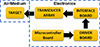 |
Figure 1 Block diagram of the ultrasonic transducer system. |
A significant effort was spent on the Transducer Array block shown in Figure 1. In the next section, we specify the process of designing a specific geometry and pertinent simulation results as applicable.
2.1 Uniform Rectangular Array (URA)
A single transducer element within a 2D array can be modeled as a rectangular piston source while it emits a spherically spreading acoustic wave [9]. This pressure amplitude of this wave can be determined by the Rayleigh–Sommerfeld integral. A detailed derivation of analytical expression of the Rayleigh–Sommerfeld integral is presented in Appendix . This expression can be converted into numerical form for practical evaluation of time delays to simulate the array. Figure 2 shows a single transducer element with dimensions lx × ly having p equal segments in x-dir and q equal segments in y-dir. The lengths of each of these segments can be calculated as lx/p and ly/q in the x-dir and y-dir, respectively. Now, the centroid or the geometric center (xpc, yqc) of the pq-th segment can be defined as,
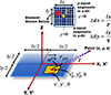 |
Figure 2 Parameters for Rayleigh–Sommerfeld integral of a single transducer element showing the segment centroid and the offset of the evaluation point (x, y, z). |
![Mathematical equation: $$ \begin{aligned} \begin{aligned} x_p^c&= - l_x/2 + \mathrm{\Delta } d_x [ p - 1/2 ] \quad p = 1,\ldots , P \\ y_p^c&= - l_y/2 + \mathrm{\Delta } d_y [ q - 1/2 ] \quad q = 1,\ldots , Q. \end{aligned} \end{aligned} $$](/articles/aacus/full_html/2026/01/aacus250065/aacus250065-eq1.gif) (1)
(1)
Assume a unit vector u p q along the axis from the above centroid to a random point (x, y, z) above the transducer plane and a random point in the segment (x′,y′,z = 0). If the 2D array has a total of n = (1, 2, …, L 1) elements in x-dir and l = (1, 2, …, L 2) in y-dir, the pressure field of the entire array with time delays Δt n l can now be written as,
 (2)
(2)
where the pressure of a single element within the multiple point source model can be described as,
 (3)
(3)
Here,
![Mathematical equation: $$ \begin{aligned} r_{pq}&= \sqrt{\left[ \left( x - x_{p}^{c} - e_{nx} \right)^{2} + \left(y - y_{q}^{c} - e_{ly}\right)^{2} + z^{2} \right]} \\ u_x^{pq}&=\left(x-x_p^c-e_{nx}\right)/r_{pq} \\ u_y^{pq}&=\left(y-y_q^c-e_{ly} \right)/r_{pq} \end{aligned} $$](/articles/aacus/full_html/2026/01/aacus250065/aacus250065-eq4.gif)
where, e n x and e l y are offsets of the centroid of the single element from the center of the array in x-dir and y-dir, respectively. They are given as e n x = (n − (L 1 + 1)/2)S x and e l y = (l − (L 2 + 1)/2)S y , where S x and S y are array pitches in x-dir and y-dir respectively. The implementation of (1)–(3) requires (a) generation of the time delays, (b) normalized pressure for a single element, and (c) normalized pressure for the entire array. The algorithm we developed computes these values for a single frequency, which is the frequency of the transducer used in the experiment and gives the results as the spatial Fourier transform of the system with k x , k y , k z as Fourier spatial frequency components. Note that (2) represents spatial spectrum of the pressure field. As the acoustic pressure wave propagates through the fluidic medium (e.g. air or water), the analytical model predicts how the pressure field varies at different heights. Consequently, if specific time delays are applied, a high-pressure focal region can be created.
2.1.1 Simulation results
To begin with, 1D 8-element array was simulated using the equations of radiating surface with 2D Rayleigh–Sommerfeld integral for each transducer acting as a piston source. Figure 3 shows the normalized pressure in air as it increases from low (blue) to high (red). The focal point with maximum pressure field value was observed at 7.8 cm above the plane of the array where x = 0 marks the center of the array.
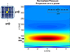 |
Figure 3 Normalized pressure field wave simulation in air for 1D 8-element array. |
Here, the center to center pitch is 1.25 cm with each element length = 1 cm. Next, 8 × 8 rectangular grid pattern was simulated with z = 1 to 142 mm in steps of 1 mm. Figure 4 shows the normalized pressure wave in air and its projection on x–y plane at three separate distances: z = 1 mm, 71 mm, and z = 142 mm. In the simulations shown in Figures 3 and 4, the array elements were fed with continuous sine wave with different delays without any apodization method to reduce side lobes. It is also important to note that the pressure field wave patterns depend on the dimensions of an individual element, the center-to-center pitch between the elements, and the gap between the elements. We picked all of the above dimensions to imitate our potential experimental setup as best as possible.
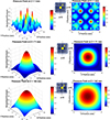 |
Figure 4 Normalized pressure field wave simulation in air for 2D 8 × 8 Uniform Rectangular Array (URA) using Rayleigh–Sommerfeld Integral: (a) z = 1 mm, (b) z = 71 mm, (c) z = 142 mm. The peak pressure appears at 71 mm. |
The dimensions were kept the same as 1D array; the exact focal point with maximum pressure amplitude value was observed at 70.85 mm above the array plane from the magnitude of the normalized pressure field and its projection on x–y plane. It was observed that the pressure value approximately halved at the edges of the plane (e.g. y = +4.88 cm and y = −4.88 cm). This is expected given the behavior of 1D array shown in Figure 3, i.e. the pressure field tends to spread out at the edges. Similar behaviour was observed while sweeping the distance directly above the center up to 142 mm. We also note that the array exhibits multiple pressure peaks at z = 1 mm, albeit of being small, progressing into a single sharpest peak at z = 70.85 mm, and then diverging away from the center at z = 142 mm (note that Fig. 4 shows the normalized pressure profile as seen on the 8 × 8 xy grid and not the value of the pressure in z dir since the algorithm requires one to select z value first). Although the experimental setup may vary a bit from these dimensions, it would provide us with a good starting point as to where we should expect the peak pressure value. These simulations, based on analytical expressions and numerical implementation, compute the total pressure in the x–y plane projected into the z-direction, requiring a specified z-distance in the coding algorithm. This approach enables visualization of wave focusing at different depths, but it would be equally beneficial to identify the optimal pressure profile across the entire z-range. To achieve this, the same 8 × 8 URA grid was simulated in MATLAB’s Phased Array System Toolbox with the sonar transducer projector option as shown in Figure 5. This simulation also helped us determine the optimal distance for maximum pressure while minimizing sidelobes with the 3D directivity pattern. Table 1 shows the parameter values for the simulations shown in Figures 4 and 5. Figure 5 shows two different directivity patterns with top set showing no apodization applied and the bottom set with Hamming tapering enabled. It is clear that apodization is beneficial in reducing the side lobes. However, the peak directivity reduces from 7.66 dBi to 5.98 dBi. This gives us a clear choice between selecting time delays with/without apodization; here, we opted for no apodization in the experimental prototype to avoid creating peak reduction. Results shown in Figures 4 and 5 are complementary and are in good agreement with one another in regards to the main lobe, which is generated directly above the center of the plane. We note that the directivity of main lobe reduces further by −12 dBi if the side-lobe taper option is turned on with other types of windows, e.g. Kaiser or Chebyshev.
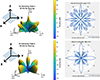 |
Figure 5 3D and 2D directivity patterns simulated with no apodization (top) and Hamming taper (bottom): back-baffle was enabled, and propagation speed was set to 343 m/s (air). |
Parameters for URA simulation.
2.2 Concentric Circular Array (CCA)
To explore an alternative to the URA design, we undertook another design topology. In this design, an array is formed with concentric rings of ultrasonic transducers with increasing numbers and spacing between the rings where each ring contains transducer elements evenly spaced around the circumference. Here, pressure field derivation needs to account for the radial and angular distribution of elements. Let r m = radius of the m-th ring, N m = the number of elements in the m-th ring, M = total number of rings. The transducer plane is defined in terms of the radial coordinate r and the azimuthal angle φ with the pressure summed along the z axis above this plane. Thus, the pressure field of the entire array with relative time delays Δtmn in cylindrical coordinates can be described as,
 (4)
(4)
where the pressure of a single element is defined as,
 (5)
(5)
Here, a = radius of a single transducer (e.g. 10 mm), k = wave number, v o (ω) = angular frequency dependent velocity magnitude (assumed to be one in simulations), C m n = weighting or apodization factor for each element, M = total number of concentric rings, J 1 = first-order Bessel function. Let angular position of each element in each ring be θ m n = 2π n/N m . Then the distance from an element to a point in the cylindrical coordinate system is,
and the angular term inside the Bessel function is,

Note that the expression in (5) includes scaling and weighting, Bessel term, phase delay, and spherical spreading, which take into account each element’s contribution. These actions/terms are described in detail as follows:
-
(1)
Scaling: The complete contribution of each element is weighted by C m n and scaled by the constant ρ c v o (ω)/2π and the element integration term ( − i k π a 2).
-
(2)
Bessel function term: The factor 2J 1(k asinθ m n ) / (k asinθ m n ) is included to describe how the finite size of the circular transducer shapes the acoustic pressure beam. It predicts a central main lobe surrounded by side lobes. The argument of the function k asinθ m n shows that the beam pattern depends on the wavenumber (and hence frequency) and the transducer radius a and the angle θ. As θ increases (moving away from the central axis), the function decreases and exhibits oscillatory behaviour.
-
(3)
Phase delay: The term e i ωΔt m n represents the propagation delay from the element to the observation point. Here, relative phase delay Δt m n = (r m n − z)/c. In terms of practice, the phase delay allows one to steer or focus the beam.
-
(4)
Spherical spreading: The exponential term e i k r m n /r m n represents the spherical spreading, i.e. the decay and phase shift with distance from the element to the point of interest in far-field.
The analytical model shown in (4) and (5) describes how the wave propagates through the fluid and predicts how the pressure field varies at different heights given the focusing delays.
2.2.1 Simulation results
The numerical simulations based on (4) and (5) were performed. Once again, pressure amplitude was calculated at different heights above the transducer plane with z = 83 mm yielding the peak pressure. Figure 6 shows the simulations of normalized pressure at z = 1 mm, 83 mm, and 161 mm. Figure 7 shows 3D and 2D directivity patterns simulated in MATLAB’s Phased Array System Toolbox with sonar transducer projector option enabled. Here, the top chart shows the simulation with ring radii of 7 cm, 13.5 cm, 27 cm, and 40.5 cm and the bottom chart shows the ring radii of 10 cm, 20 cm, 30 cm, and 40 cm. Both ring to ring spacing aka ring radii values yield approximately same peak value of 20 dBi, which is substantially higher than the URA peak value. We note that the uneven spacing value in the top figure comes from PCB design consideration and physical size of the transducer as dictated by the manufacturer. Table 2 shows various parameters used in CCA simulation.
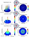 |
Figure 6 Normalized pressure field wave simulation in air for 2D Concentric Circular Array (CCA) using Rayleigh–Sommerfeld Integral: (a) z = 1 mm, (b) z = 83 mm, (c) z = 161 mm. The peak pressure appears at 83 mm. |
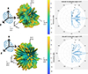 |
Figure 7 3D and 2D Directivity Patterns Simulated with ring radii of 7 cm, 13.5 cm, 27 cm, and 40.5 cm (top) and ring radii of 10 cm, 20 cm, 30 cm, and 40 cm (bottom): back-baffle was enabled, and propagation speed was set to 343 m/s (air). Uneven spacing reduces sidelobes while preserving central lobe amplitude. The central lobe level stays constant around 20 dBi. |
Parameters for CCA simulation.
Next, a series of simulations were performed to determine the dependence of acoustic pressure generated by the array on element to element spacing and ring to ring spacing as shown in Figures 8 and 9. It is quite evident that pressure amplitude peaks at two prominent values above the transducer plane, first one at 49.5 mm and second one at 83 mm, which is the maximum of the two. Figure 8 shows the comparison of max pressure values with two different ring to ring spacing for a total of four rings. These pressure values were determined by finding the maximum value within a radius of 20 mm in the center lobe in Figure 6. The first set, i.e. 10 mm, 20 mm, 30 mm, 40 mm can be considered as linearly increasing ring radii values with similar order of progression. The second set of ring radii values, i.e., 7 mm, 13.5 mm, 27 mm, 40.5 mm, was determined by considering a maximum layout size with 10 cm diameter and the size of the actual transducer with 10 mm radius. It can be readily observed that for the element to element spacing values between 14 mm and 16 mm, the max pressure values are nearly identical. Hence we chose the second set of spacings in the actual PCB layout (see inset of Fig. 9). The max peak was observed at z = 83 mm above the transducer plane. The number of elements per ring were determined as Nm = 2πrm/s, where rm = individual ring radius and s = element to element spacing.
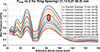 |
Figure 8 Maximum pressure P max vs distance Z for ring to ring spacing of [7, 13.5, 27, 40.5] mm for varying element-to-element spacing. Note that the peak values occur at approximately 83 mm. The red oval represents the element to element spacing highlighted in Figure 9. |
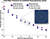 |
Figure 9 The peak max pressure value obtained from the data shown in Figure 8 for uneven ring to ring spacing compared to even ring to ring spacing values: the element to element spacing between 14 and 16 mm exhibits a good match between the two types of rings. Here, the highlighted spacing values were chosen in the PCB layout shown in the inset. |
3 Characterization of transducer arrays
The generic system shown in Figure 1 was implemented to characterize the pressure field of the two ultrasonic transducer arrays: the Uniform Rectangular Array (URA) and the Concentric Circular Array (CCA) as discussed in the previous section. In general, ultrasonic transducers act as spatial frequency sources, where each transducer in the array contributes to the overall spatial frequency spectrum of the emitted wave. The aperture function, determined by the spatial layout of transducers, defines the Fourier spectrum of the emitted wavefield. In the previous section, we described the acoustic wave propagation in the frequency domain using the Fourier-transformed solution, which explains how spatial frequencies propagate through the medium. Consequently, the pressure field at any given point (x, y, z) can be viewed as a summation of plane waves with distinct spatial frequency components. This framework extends naturally to the experimental domain, where a matching receiver transducer (Murata MA40S4R) was used to measure the pressure field at a given location. Thus, the measured signal corresponds to a spatially filtered inverse Fourier transform of the emitted wave. By systematically scanning the receiver across different positions, we effectively sample the inverse Fourier transform of the transmitted field, allowing us to reconstruct the measured acoustic pressure distribution. To realize this measurement approach, we developed an experimental setup with a modular, bottom-up electronic topology with a microcontroller board, a driver board, a transducer board, which are briefly described next.
3.1 Microcontroller board
A microcontroller board (Arduino MEGA) was programmed such that its digital I/O ports can switch between LOW (0 V) and HIGH (5 V). The switching rate was fixed and created a square output signal at 40 kHz. The time delay between the ports and sequencing between the ports created the desired interference pattern. The time delays were determined from the simulation of URA and CCA.
3.2 Driver board
Next, the driver board was designed to increase the voltage level of the output signal from the microcontroller to 20 V and to provide current as required by the transducers at that voltage level. The driver boards were designed and fabricated depending on the type of the transducer geometry (e.g. rectangular, circular). This part of the transducer system was challenging in that the selection of driver IC (Microchip Tech MIC4127YME) and pertinent electronics play a major role in the type and level of the waveform produced by the individual transducers. The driver IC had dual power MOSFETs providing current levels up to 1.5 A [10]. Depending on the driver IC and the driver board configuration, an interface board was used between the driver board and the transducer array board to facilitate interconnections between the two boards. Before connecting the transducer board to this board, we verified both the programmed time delays on Agilent 16902A logic analyzer as shown in Figure 10 and the voltage levels on Siglent SDS2204x Plus digital oscilloscope.
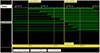 |
Figure 10 Logic analyzer verification of microcontroller timing delays before connecting the transducer array. |
3.3 Transducer array board
For the two prototypes discussed in this paper, we used the Murata MA40S4S transducer. This is a low-cost (available for ∼$5/unit in July 2024) transducer that exhibits a sharp peak of 120 dB Sound Pressure Level (SPL) at 40 kHz. The transducer has nearly symmetrical and omnidirectional beam pattern with 0 dB attenuation between −30 deg/+30 deg from the center while its max attenuation is about 20 dB attenuation on the sides between −90 deg/+90 deg from the center [11]. It has no sidelobes and serves well as a general-purpose transducer for the initial designs. Each of the transducers was checked to mark its polarity appropriately using digital oscilloscope. The negative terminals were grounded together on the PCB by connecting a ground trace from the microcontroller board. The positive terminals of each of the transducers were connected to appropriate driver output pins on the driver board. Thus, the interface between transducer board and driver board was achieved in a plug-and-play configuration. The idea was to try different transducer boards using the same driver board.
3.4 Receiver and XYZ stage
To automate pressure field measurements, we modified a Creality Ender3 3D printer, removing the print head and cooling fan thus creating our own X Y Z stage. We also designed and 3D-printed a custom holder together with readout PCB for MA40S4R transducer with sensitivity of 0.00708 V/Pa to be used as the receiver. This receiver transducer captured the transmitted signals, which were measured as voltage waveforms on Siglent SDS2204x Plus digital oscilloscope. After the data capture, each voltage waveform was processed as follows: (1) truncate the data to 1.2 ms duration window, (2) apply 4th order Elliptic bandpass filter with low and high cutoff frequencies = 20 kHz and 60 kHz, respectively, (3) subtract the mean, (4) apply Hilbert transform to detect the envelope of the voltage signal and determine the maximum value, and (5) convert the max voltage to max pressure based on the receiver sensitivity. The X Y-plane pressure field was mapped at different Z-values, leveraging the X Y Z stage’s motion control for precise, repeatable positioning of the receiver transducer. Since the receiver transducer’s output voltage corresponds to the incident pressure field, this method enables a direct experimental validation of the simulation results, providing insight into beam focusing and spatial pressure distribution.
3.5 Characterization results for URA
The PCB with 8 × 8 grid of URA was connected to 64 output driver board to drive each of the transducers individually by the microcontroller. Time delays from the simulation results were converted to machine cycles of ATmega2560 microcontroller. The transducer array was switched at 40 kHz. We observed 3 cycles of instructional delay between the time delays after measuring the response of microcontroller port pins on the logic analyzer. The original setup with 64 individual delays was greatly simplified by considering identical time delays for specific transducers based on the simulation results shown in Figure 4. For example, all four corner transducers were driven at machine cycles = 0 and all four center transducers were driven at machine cycles = 9, etc. Correspondingly, we designed and utilized an interface board between the microcontroller and the transducer board so that each driver IC output can drive 4 transducers simultaneously. We developed custom-designed prototype after experimenting with the breadboard-level implementation shown in Figure 11. We obtained the baseline experimental results of the URA in air to verify the proof of concept as shown in Figure 12. This result very closely matches the simulation result of ∼71 mm shown in Figure 4 with maximum pressure at 75 mm obtained in the experiment. The DC bias was set to 20 V and the total current draw was measured as 266 mA.
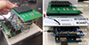 |
Figure 11 Development of 8 × 8 Uniform Rectangular Array (URA) prototype: version 1 (L) with breadboard-mounted PCBs and version 2 (R) with a stack of custom PCBs. |
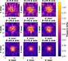 |
Figure 12 Measured pressure levels from 5 mm to 80 cm above the 8 × 8 URA: A clear focal peak is observed near z = 75 mm. Note that the spot disperses at higher values of Z as expected. |
Summary of main results.
3.6 Characterization results for CCA
The CCA prototype shown in Figure 13. In the final iteration of the design, we opted for the number of elements as 4, 8, 16, 24 with ring radii as 7.5 mm, 21.5 mm, 33.5 mm, 47.5 mm, respectively. The total number of transducers in the entire array was 52 and the element to element spacing was varied between 13.5 mm and 15 mm as necessary to fit the array appropriately with rcca = 50 mm in the perimeter. Figure 13 also shows the time delay in microseconds at the approximate location of each transducer. When focusing on a point above the array plane, all the waves must arrive at the focal point in phase. The distance from each transducer to the focal point varies. For example, the center ring has the shortest path and the outer ring has the longest path. To have constructive interference at the focal point, the idea is to compensate for these extra distances by delaying the signals such that the outer transducers are triggered earlier than the center element. In other words, the computed delay values are larger as you move inward toward the center as shown in Figure 13. Here, the MATLAB code was modified to calculate time delay values considering the physical layout of the rings with the maximum radius of 50 mm. These results are shown in Figure 14. The DC bias was set to 20 V and the total current draw was measured as 380 mA.
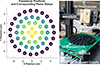 |
Figure 13 CCA Experiment Setup: CCA transducer rings and corresponding rounded time delays derived from simulations in microseconds for activating each transducer (L). This scheme was implemented for the results shown in Figure 14, as measured from CCA PCB stack on X Y Z stage with receiver PCB (R). |
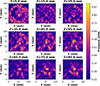 |
Figure 14 Measured pressure levels from 5 mm to 85 cm above the 52 element CCA: A weak peak appears near z = 65 mm, however the spot disperses at larger distances. |
After few other iterations of the microcontroller code with alternate time delays, it became clear that the URA outperformed CCA not only in terms of total power consumption but also maximum peak pressure. The CCA design is also bit more challenging in terms of the placement of rings, number of rings, element-to-element spacing, etc. Table 3 summarizes the key results from the design, simulation, and experiments of both URA and CCA. The acoustic intensity corresponding to the measured peak pressures was estimated using I = Pmax2/(2ρc), where Pmax = peak pressure, ρ = density of air = 1.225 kg/m3, and c = speed of sound in air = 343 m/s. It is important to note that all simulations and experiments were performed in air. Water or lung tissue would have higher acoustic impedance and attenuation coefficient. Here, the higher impedance would result in increased reflection at boundaries, while greater attenuation and absorption would lead to lower peak pressures and shallower focal regions thus changing the pressure field, focal distance, and intensity. Also note that water/tissue will exhibit rapid absorption at higher frequencies. These effects will be addressed in future work as we transition toward a high frequency design for therapeutic use in a biological system.
4 Summary and future work
The list below gives an overview of the work to be performed as this research is continued forward:
-
(1)
Extend the transducer operation into the medical ultrasound frequency band (1–4 MHz) to target specific applications more effectively.
-
(2)
Develop an integrated, single-PCB design that combines the microcontroller PCB, driver PCB, interface, and transducer PCB.
-
(3)
Explore novel geometries beyond the current URA and CCA designs, including bowl-shaped rigid arrays and conformal/wearable arrays. These configurations may enhance beam steering, focusing, and patient-specific solutions.
-
(4)
For cell model to be used in either CF or other disease modality, establish a database of viscosity samples (e.g. glycerol, artificial sputum, mucus) to systematically document how ultrasound influences their properties and evaluate key parameters such as pulse repetition rate, pressure level, and specific frequency over a range of distances.
-
(5)
Investigate the effects of electronically coupled transducer arrays with non-linear behavior: the aim is to leverage the synchronization properties to develop agile and responsive systems capable of adapting to varying therapeutic requirements.
Acknowledgments
The authors would like to thank Dr. Chris Capaldo and his students in the Department of Biology at HPU for their valuable contributions to the biological aspects of the project, particularly in developing the cell model and applications to specific disease modality to be used as a reference point, as well as for their insightful discussions.
Funding
This work was supported by undergraduate Student Research Experience (SRE) funded by the IDeA Networks of Biomedical Research Excellence (INBRE) and Islands of Opportunity Alliance–Louis Stokes Alliances for Minority Participation (IOA-LSAMP) at HPU.
Conflicts of interest
The authors declare no conflicts of interest.
Data availability statement
The measured data is in Zenodo, under the reference [12]. Any other information including Arduino codes, PCB gerber les, are available on request from the corresponding author.
References
- J.P. Clancy, C.U. Cotton, S.H. Donaldson, G.M. Solomon, D.R. VanDevanter, M.P. Boyle, M. Gentzsch, J.A. Nick, B. Illek, J.C. Wallenburg, E.J. Sorscher: CFTR modulator theratyping: current status, gaps and future directions. Journal of Cystic Fibrosis 18 (2019) 22–34. [Google Scholar]
- C. Huang, H. Zhang, R. Bai: Advances in ultrasound-targeted microbubble-mediated gene therapy for liver fibrosis. Acta Pharmaceutica Sinica 7 (2017) 447–452. [Google Scholar]
- M. Anzidei, A. Napoli, F. Sandolo, B.C. Marincola, M. Di Martino, P. Berloco, S. Bosco, M. Bezzi, C. Catalano: Magnetic resonance-guided focused ultrasound ablation in abdominal moving organs: a feasibility study in selected cases of pancreatic and liver cancer. Cardiovascular and Interventional Radiology 37 (2014) 1611–1617. [Google Scholar]
- M. Rauch, M. Marinova, H.H. Schild, H. Strunk: High intensity focused ultrasound for the treatment of advanced liver cancer. Digestive and Liver Disease 47 (2015) 989–990. [Google Scholar]
- H. Wei, L. Shi, J. Zhang, Y. Xia, J. Cuan, Y. Zhang, W. Li, A. Yan, X. Jiang, M.F. Lang, J. Sun: High-intensity focused ultrasound leads to histopathologic changes of the inferior turbinate mucosa with allergic inflammation. Ultrasound in Medicine & Biology 40 (2014) 2425–2430. [Google Scholar]
- R. Zhang, X. Chen, M. Feng, L. Chen, H. Wang: Study on focal distance of II type uterine fibroids under mucous membrane treated by high intensity focused ultrasound ablation. Chinese Journal of Primary Medicine and Pharmacy 23 (2016) 1835–1840. [Google Scholar]
- D.L. Miller, N.B. Smith, M.R. Bailey, G.J. Czarnota, K. Hynynen, I.R.S. Makin, Bioeffects Committee of the American Institute of Ultrasound in Medicine: Overview of therapeutic ultrasound applications and safety considerations. Journal of Ultrasound in Medicine 31 (2012) 623–634. [Google Scholar]
- A. Marzo, T. Corkett, B.W. Drinkwater: Ultraino: an open phased-array system for narrowband airborne ultrasound transmission. IEEE Transactions on Ultrasonics, Ferroelectrics, and Frequency Control 65 (2018) 102–111. [Google Scholar]
- L. Schmerr: Fundamentals of Ultrasonic Phased Arrays. Springer, 2015. [Google Scholar]
- Microchip Technology: MIC4127 Dual 1.5A-Peak low-side MOSFET drivers in advanced packaging. MIC4127 datasheet, 2019. [Google Scholar]
- Murata Inc: MA40S4S ultrasonic transducer. MA40S4S datasheet, 2015. [Google Scholar]
- S. Naik: Measured dataset for URA and CCA. Zenodo, 2025. https://zenodo.org/records/16730183. [Google Scholar]
Appendix A
Analytical expressions
Acoustic pressure field of a single element in a 2-D array
First principles equations in acoustics describe the pressure field in a fluid like air or water based on the continuity equation and momentum equation. Hence, the pressure field p(r, t) of a single element in a 2D array, as shown in Figure A.1 (L), in the fluid will satisfy the spatiotemporal 3D wave equation,
 (A.1)
(A.1)
where c = wave speed with EB = bulk modulus and ρ = density of the medium.
After taking the Fourier Transform of the above equation and representing wave propagation in frequency domain, we arrive at the general solution of 3D Helmholtz equation on the plane z = 0 as,
 (A.2)
(A.2)
where P(kx, ky) is the 2D spatial Fourier transform representing the amplitude term and is given as,
 (A.3)
(A.3)
In the transform pair equations (A.2) and (A.3), kx = kcosϕsinθ and ky = ksinϕsinθ with k = ω/c, where ω = angular frequency and c = speed of the wave in the medium, is defined in spherical coordinates as shown in Figure A.1 (R) below. Note that the transducer element is assumed to be embedded in motionless plane called rigid baffle. In this model, the normal velocity is zero everywhere else except the transducer element.
The frequency domain version of the spatial transform of the pressure wave is useful in analyzing and simulating beam patterns because it provides a comprehensive understanding of how different frequencies contribute to the spatial distribution of ultrasonic energy. Consequently, equation (A.2) gives us the 2D spatial Fourier transform of pressure field on z = 0 plane of a 3D angular plane wave spectrum in spherical coordinates. The z-component of the velocity on z = 0 plane is given by,
 (A.4)
(A.4)
where V(kx, ky) is the 2D spatial Fourier transform of z-velocity and is given as,
 (A.5)
(A.5)
Note that the generalized form of equation (A.2) has nonzero z component. The Fourier transform of such a pressure field in terms of velocity can be written by using equation (A.5) as,
 (A.6)
(A.6)
After applying the convolution theorem and assuming that the velocity field is constant vz = vo(ω) as shown in Figure A.1 (L), we arrive at the Rayleigh–Sommerfeld integral for the single transducer element as a piston model,
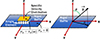 |
Figure A.1 Single transducer element as a velocity source using piston model as the face of the element (L) and Wave number vector k in spherical coordinates (R). |
 (A.7)
(A.7)
A = surface area of the transducer element, and the distance from the element to a pressure point is given by  .
.
Appendix B
Additional experimental details
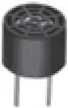 |
Figure B.1 Picture of the Murata MA40S4S transducer. |
 |
Figure B.2 Directivity of the Murata MA40S4S transducer. |
 |
Figure B.3 Picture of the MIC4127YME driver IC. |
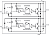 |
Figure B.4 Functional block diagram of the MIC4127YME driver IC. |
Cite this article as: Naik S. Horikawa J. Lyne L. Dimaunahan R. Aquino G. … Hara M. 2026. Design and characterization of ultrasonic transducer array system for targeted non-invasive treatment. Acta Acustica, 10, 3. https://doi.org/10.1051/aacus/2025068.
All Tables
All Figures
|
Figure 1 Block diagram of the ultrasonic transducer system. |
| In the text | |
|
Figure 2 Parameters for Rayleigh–Sommerfeld integral of a single transducer element showing the segment centroid and the offset of the evaluation point (x, y, z). |
| In the text | |
|
Figure 3 Normalized pressure field wave simulation in air for 1D 8-element array. |
| In the text | |
|
Figure 4 Normalized pressure field wave simulation in air for 2D 8 × 8 Uniform Rectangular Array (URA) using Rayleigh–Sommerfeld Integral: (a) z = 1 mm, (b) z = 71 mm, (c) z = 142 mm. The peak pressure appears at 71 mm. |
| In the text | |
|
Figure 5 3D and 2D directivity patterns simulated with no apodization (top) and Hamming taper (bottom): back-baffle was enabled, and propagation speed was set to 343 m/s (air). |
| In the text | |
|
Figure 6 Normalized pressure field wave simulation in air for 2D Concentric Circular Array (CCA) using Rayleigh–Sommerfeld Integral: (a) z = 1 mm, (b) z = 83 mm, (c) z = 161 mm. The peak pressure appears at 83 mm. |
| In the text | |
|
Figure 7 3D and 2D Directivity Patterns Simulated with ring radii of 7 cm, 13.5 cm, 27 cm, and 40.5 cm (top) and ring radii of 10 cm, 20 cm, 30 cm, and 40 cm (bottom): back-baffle was enabled, and propagation speed was set to 343 m/s (air). Uneven spacing reduces sidelobes while preserving central lobe amplitude. The central lobe level stays constant around 20 dBi. |
| In the text | |
|
Figure 8 Maximum pressure P max vs distance Z for ring to ring spacing of [7, 13.5, 27, 40.5] mm for varying element-to-element spacing. Note that the peak values occur at approximately 83 mm. The red oval represents the element to element spacing highlighted in Figure 9. |
| In the text | |
|
Figure 9 The peak max pressure value obtained from the data shown in Figure 8 for uneven ring to ring spacing compared to even ring to ring spacing values: the element to element spacing between 14 and 16 mm exhibits a good match between the two types of rings. Here, the highlighted spacing values were chosen in the PCB layout shown in the inset. |
| In the text | |
|
Figure 10 Logic analyzer verification of microcontroller timing delays before connecting the transducer array. |
| In the text | |
|
Figure 11 Development of 8 × 8 Uniform Rectangular Array (URA) prototype: version 1 (L) with breadboard-mounted PCBs and version 2 (R) with a stack of custom PCBs. |
| In the text | |
|
Figure 12 Measured pressure levels from 5 mm to 80 cm above the 8 × 8 URA: A clear focal peak is observed near z = 75 mm. Note that the spot disperses at higher values of Z as expected. |
| In the text | |
|
Figure 13 CCA Experiment Setup: CCA transducer rings and corresponding rounded time delays derived from simulations in microseconds for activating each transducer (L). This scheme was implemented for the results shown in Figure 14, as measured from CCA PCB stack on X Y Z stage with receiver PCB (R). |
| In the text | |
|
Figure 14 Measured pressure levels from 5 mm to 85 cm above the 52 element CCA: A weak peak appears near z = 65 mm, however the spot disperses at larger distances. |
| In the text | |
|
Figure A.1 Single transducer element as a velocity source using piston model as the face of the element (L) and Wave number vector k in spherical coordinates (R). |
| In the text | |
|
Figure B.1 Picture of the Murata MA40S4S transducer. |
| In the text | |
|
Figure B.2 Directivity of the Murata MA40S4S transducer. |
| In the text | |
|
Figure B.3 Picture of the MIC4127YME driver IC. |
| In the text | |
|
Figure B.4 Functional block diagram of the MIC4127YME driver IC. |
| In the text | |
Current usage metrics show cumulative count of Article Views (full-text article views including HTML views, PDF and ePub downloads, according to the available data) and Abstracts Views on Vision4Press platform.
Data correspond to usage on the plateform after 2015. The current usage metrics is available 48-96 hours after online publication and is updated daily on week days.
Initial download of the metrics may take a while.