| Issue |
Acta Acust.
Volume 9, 2025
|
|
|---|---|---|
| Article Number | 20 | |
| Number of page(s) | 11 | |
| Section | Computational and Numerical Acoustics | |
| DOI | https://doi.org/10.1051/aacus/2024078 | |
| Published online | 07 March 2025 | |
Scientific Article
Modelling of superposition in 2D linear acoustic wave problems using Fourier neural operator networks
1
AudioLab, School of Physics, Engineering and Technology, University of York, Heslington, York YO10 5DD, UK
2
Department of Computer Science, Acoustics Lab, Aalto University, P.O. Box 15400, FI-00076 Aalto, Finland
* Corresponding author: michael.middleton@york.ac.uk
Received:
16
September
2024
Accepted:
28
October
2024
A method of solving the 2D acoustic wave equation using Fourier Neural Operator (FNO) networks is presented. Various scenarios including wave superposition are considered, including the modelling of multiple simultaneous sound sources, reflections from domain boundaries and diffraction from randomly-positioned and sized rectangular objects. Training, testing and ground-truth data is produced using the acoustic Finite-Difference Time-Domain (FDTD) method. FNO is selected as the neural architecture as the network architecture requires relatively little memory compared to some other operator network designs. The number of training epochs and the size of training datasets were chosen to be small to test the convergence properties of FNO in challenging learning conditions. FNO networks are shown to be time-efficient means of simulating wave propagation in a 2D domain compared to FDTD, operating 25 × faster in some cases. Furthermore, the FNO network is demonstrated as an effective means of data compression, storing a 24.4 GB training dataset as a 15.5 MB set of network weights.
Key words: Machine learning / Neural networks / Linear acoustics / Reflections / Generalisation
© The Author(s), Published by EDP Sciences, 2025
 This is an Open Access article distributed under the terms of the Creative Commons Attribution License (https://creativecommons.org/licenses/by/4.0), which permits unrestricted use, distribution, and reproduction in any medium, provided the original work is properly cited.
1 Introduction
The Finite Difference Time Domain (FDTD) method [1, 2] is a well established numerical method within the field of room acoustic simulation, and has been long studied for its relatively simple implementation and flexibility, ability to produce broadband simulations in one single pass and relative ease of computational parallelisation for solving larger problem domains [3]. However, despite these benefits, it is still inefficient in terms of computation time and memory use for very large acoustic spaces, and real-time implementations are very limited [4, 5].
More recently, neural network approaches have been used to solve scientific problems expressed by partial differential equations (PDEs) [6–9]. This has included some limited application for acoustics problems [10, 11]. One such approach, using a Fourier Neural Operator (FNO) for scientific deep learning for simple 2D acoustic problems is adopted in this paper with training data sourced from an explicit compact FDTD numerical solution to the 2D linear wave equation. The FNO is capable of modelling wave propagation for acoustics problems when provided with several initial steps of FDTD simulation data as an input function to the network [10]. FNO networks demonstrate strong generalisation in comparison to other scientific deep learning approaches such as Physics-Informed Neural Networks (PINNs) [6, 7]. Problems unseen by the network during training are predicted at a similar level of error to solutions in the training dataset.
Once an FNO has been trained, the simulation process is reduced to a simple, and usually efficient, linear algebraic process, potentially improving computational efficiency and lowering simulation times. Furthermore, as the FNO architecture displays good generalisation, it would implicitly represent wave behaviour when excited at any point within the domain it has been trained on, eliminating the need to store a large amount of simulated data.
The work presented here is an extension of previously published work by the authors [10]. In this previous paper, an FNO network was used to model 2D wave propagation over time for a square free-field domain with an excitation source that could be positioned arbitrarily within the domain boundaries. The method was tested by varying the amount of time domain input data used for training the network to obtain an output that compared well with a FDTD baseline solution. It was discovered that FNO networks could model single-source solutions well with a maximum observed input-to-output temporal data ratio of up to 1 input time-step to 16 output time-steps.
This paper develops these techniques further by testing this FNO approach under different simulation conditions. Here, up to four arbitrarily placed simultaneous sound sources are now considered in one set of experiments. Specular reflections and diffraction from a randomly-positioned block are modelled by FNO networks in a second set. It is demonstrated that FNO can solve both problem scenarios well, generalising to any set of 1–4 sound sources in the multi-source experiments accurately. In experiments involving scattering, the reflective object is rectangular and allowed to be one of four sizes. It is further demonstrated that FNO can distinguish the size of this object well, along with its position.
The FNO is assessed on data outside of its training set and the network architecture demonstrates good generalisation properties. Data obtained from two different FDTD stencils commonly used in room acoustics literature is used to train and evaluate the FNOs; the Standard Rectilinear (SRL) [1] and the Interpolated Wideband (IWB) [12] stencils. In addition, a 1.25 kHz lowpass filter is used to band-limit the data prior to training the FNO network. The resulting 2D acoustic test simulations presented demonstrate an FNO model that can be trained using small FDTD training datasets, that can generalise across initial conditions and gives efficient and consistent results at run-time when presented with unseen input data.
2 Background
The 2D linear acoustic wave equation is a hyperbolic partial differential equation (PDE) defining the acoustic pressure within a medium as a function of second-order spatial and temporal partial derivatives (∂x2, ∂y2, ∂t2). It is presented in equation (1), in terms of u(x, y, t), where c is the speed of wave propagation.
Various boundary conditions can be considered and applied to terminate the medium. Typically, in room acoustics problems, it is assumed that boundaries are frequency independent and locally reacting, such that the vibration of the boundary itself is not considered, with the general continuous boundary condition defined as:
where n is the outward-pointing unit normal vector to the boundary surface and ξ represents the specific acoustic impedance of the boundary surface.
2.1 2D acoustic finite-difference time domain simulation
The general compact 2D acoustic FDTD scheme is provided in equation (3) where the Δ2 operators represent the second-order central difference scheme for the relevant dimension [1]. The SRL stencil is retrieved when a = 0 and the IWB stencil is obtained when  .
.
![$$ [1+a({\delta }_x^2+{\delta }_y^2)+{a}^2{\delta }_x^2{\delta }_y^2]{\delta }_t^2{u}_{x,y}^t={\lambda }^2[({\delta }_x^2+{\delta }_y^2)+b{\delta }_x^2{\delta }_y^2]{u}_{x,y}^t $$](/articles/aacus/full_html/2025/01/aacus240111/aacus240111-eq4.gif)
Numerical dispersion error in FDTD simulations appears as phase distortions in the simulated data, being the consequence of quantising the continuous domain data into a discrete set. Its impact can be mitigated by using finer domain sampling densities [13]. Different stencil functions within the FDTD update scheme can be used to manage dispersion error distribution. Interpolated stencils [12] spread the error across the domain isotropically, reducing the directional impact of error in comparison to rectilinear stencils.
It is possible to approximate the value of u(x, y, t) in two spatial dimensions by solving the wave equation using a numerical approach such as FDTD. FDTD has received considerable research interest in acoustic simulation, making it a well-understood and easily implemented method of solving the wave equation capable of simulating a broad-band acoustic response [2, 4, 14, 15]. Hence, FDTD has been chosen to produce training data for the FNO networks used in this paper.
The SRL and IWB FDTD stencil functions, which define how pressure at a spatio-temporal point is computed from surrounding pressure values, are used to simulate the FDTD data. SRL was chosen as it is the simplest stencil function, sampling 4 spatially adjacent points, whilst the IWB stencil was selected for its isotropic dispersion error pattern compared to SRL [2, 12].
2.2 Fourier neural operator networks
The FNO is a type of artificial neural network used in scientific deep learning [7]. Rather than supplying a variable (such as a coordinate) to the network and predicting a quantity associated to that value (see PINNs [6, 16, 17]), operator networks map from one functional space to another [7]. A function, in this case, a limited set of initial time-steps from the acoustic FDTD method, is passed to the FNO. Another function, the continued wave propagation after the input time-steps, is predicted. FNO has been used to solve problems such as wave equations [18, 19], Navier-Stokes problems [7] and fluid flows [20]. Unlike PINNs, FNO exhibits excellent generalisation when trained on a dataset of similar physical problems with variable initial or boundary conditions [7, 10].
FNO networks learn local and non-local features by performing efficient convolution over the whole domain by multiplying the signal spectrum with a matrix of weights. Equation (4) describes the signal transformation that occurs in the Fourier convolution layer as represented in Figure 1, where s is the input signal from the proceeding layer, W, B are matrices of adjustable complex-valued weights representing weight and bias terms respectively,  ,
,  are operators for the FFT and inverse FFT transforms respectively and q is the length of the FFT spectrum in bins divided by 2 rounded up to the nearest integer. σ is a non-linear activation term; the Gaussian-error Linear Unit (GeLU) function [21] is suggested for FNO learning [7]. A graphical representation of the flow of data through the FNO network is shown in Figure 1, where z is the data batch size, L is the length of the temporal dimension and I is the number of input time-steps to the network.
![$$ g=\sigma (s+\mathcal{IF}(\mathcal{F}(s{)}_{[1...q]}\odot \mathbf{W}+\mathbf{B})) $$](/articles/aacus/full_html/2025/01/aacus240111/aacus240111-eq7.gif)
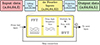 |
Figure 1 A representation of the FNO network architecture. Layer shapes in tensors are shown in parentheses. The transformed signal is usually truncated with high-frequency FFT bins discarded as a regularisation measure [7]. |
Skip connections are used between layers, where the input s is summed with the layer output g. Skip connections are used to model non-periodic boundary conditions by allowing weights to be trained without being transformed by the FFT [7]. Additionally, skip connections avoid singularities forming when incoming or outgoing weights from a neuron reduce to zero. Singularities cause neural network training to slow down significantly and are broken by skip connections as features from previous layers are preserved [22]. Finally, the signal is transformed by a nonlinear activation function and passed to subsequent layers.
In the complete FNO network, two additional fully-connected layers are incorporated into the design. They are the lifting and projection layers which proceed and follow the stack of Fourier layers respectively. The lifting layer increases the dimensionality of the input data to allow for more spectral information to be learned from the signal. Similarly, the projection layer lowers the dimensionality of the output from the Fourier layers to what is required for the network output. As these layers are parameterised with trainable weights, this process is not analogous to increasing the number of FFT bins within the Fourier layers.
2.3 Discussion on operator network designs
The key component of the FNO network is the Fourier convolution layers which substitute the densely connected layers found in other formulations of neural networks like CNNs [7]. As such, Fourier convolution layers have been introduced in place of densely-connected layers in Gated Recurrent Unit (GRU) networks to model time-series problems [8]. These Fourier Gated Recurrent Unit (F-GRU) networks have been used to model acoustic propagation and boundary reflections in two spatial dimensions [8], although F-GRU networks require nearly triple the parameter count of an FNO network to solve an equivalent acoustic problem. This is because the F-GRU stores the state of the network in memory allowing subsequent inputs to be affected by the present state of the system. This feature protects against instability during training by providing the system with time-domain awareness [8] but requires more computational memory to store the additional information. For this reason, FNO networks were selected for the research presented here over F-GRU.
DeepONets are another formulation of operator network that learns from sparsely-sampled data, rather than the whole domain. They have found application in room acoustic simulation problems, solving the 3D wave equation with reflective surface modelling [11]. DeepONets also allow for non-linear and deformed grids to be sampled directly, however, whilst FNO must project a non-linear sampling scheme onto a linearly-spaced grid first [23, 24]. It has been demonstrated that DeepONets and FNO are equivalent in prediction accuracy when considering smooth problems [23]. FNO networks also predict the whole acoustic field in a single pass whilst that predicted by a DeepONet solution must be constructed one point at a time [9]. FNO was selected over DeepONet for this research as the training data produced by FDTD is regularly sampled and predictions are simpler to obtain from the trained FNO network.
3 Methodology
In this paper, FNO networks are trained to predict the solution to 2D wave propagation problems when provided with a sequence of input time-steps obtained from a FDTD simulation. Accuracy of FNO predictions are quantified by computing the absolute and Mean-Squared Errors (MSE) of FNO outputs against ground-truth FDTD simulations in the time and frequency domains. Prediction times of FNO networks are also compared to the computation time of equivalent FDTD simulations.
3.1 FDTD simulation for FNO modelling
FDTD simulation was implemented in Python 3.10 using the Numpy package. The machine used to produce the FDTD data and train the FNO networks had a 12-core 3.5 GHz processor, 32 GB of RAM and an 8 GB NVidia 2060 Super GPU for parallel computation. The acoustic FDTD method operating in 2 spatial dimensions plus time was used to prepare the training and ground-truth data for the network. Four square domains are defined and considered, described in Table 1.
Simulation domain details.
Both spatial dimensions for all domains measure 64 samples. One is free-field and waves are allowed to propagate past the boundary without any reflections. It receives multiple simultaneous excitation sources and is labelled “Multi”. Waves are also allowed to pass the boundary for the “Scattering” domain, which also introduces a rectangular object into the space. This block can measure 8 × 8, 8 × 16, 16 × 8 or 16 × 16 samples in the X and Y dimensions. The object is also assumed to be perfectly smooth, reflective and stationary. Its position within the domain is random and the block is entirely contained within the domain in all examples. A third domain with reflective boundaries (labelled “Boundary”) is not a free-field space; each edge of the domain is modelled as a perfectly reflective surface with a negative reflection coefficient, inverting the phase of reflected waves with zero energy absorption. A fourth domain (“B+S”) also uses reflective boundaries defined in the same manner, plus the reflective block modelling used in the scattering domain. In discrete time, reflections from surfaces are modelled by Dirichlet boundary conditions;  .
.
For each domain, the number of input time-steps given to the FNO is defined as I, whilst the number of subsequent time-steps predicted is given as L (Table 1). Each domain also receives padding in both spatial dimensions. Where waves can pass beyond domain boundaries (multi-source and scattering), the domain is padded symmetrically by 33 samples. Where boundary reflections are modelled (boundary and B+S), domains are symmetrically padded by 1 to model the reflective surface. Padding is removed from the domain after FDTD simulation. FNO predictions are obtained for the multi-source domain by providing the FNO with the initial 16 time-steps of FDTD simulation as input data, with the remaining 64 being predicted by the network. Predictions for all other domains measure 128 time-steps in length, with 32 provided as input data to the network. Fewer overall time-steps are considered for the multi-source domain as there are no opportunities for the propagating waves to reflect from anything in the space. This causes waves to escape from the domain in relatively few time-steps, which would result in the FNO modelling silence and dispersion error for much of the prediction period if the time dimension is not reduced. For all experiments, a ratio of 1 input to 4 output time-steps are modelled by the FNO, which has previously been established to be a stable data ratio to train an FNO for acoustic modelling [10].
The speed of sound in air is assumed as c = 343 m/s with spatial and temporal sampling defined as ΔD = 0.043 m and Δt = 88.388 μm respectively. The predicted area of the domains, at 64 × 64 samples, can be calculated as 7.53 m2. The Courant number λ is defined here as  . FNO output predictions measure a signal of length 5.657 ms for the multi-source domain and 11.314 ms for all other domains. For the multi-source domain, FDTD simulations occupy 2.62 MB in working computer memory. For all other domains, FDTD simulations occupy 5.24 MB.
A Dirac pulse  (Eq. 5) is used as the excitation signal for the system initial condition. It is applied at a randomly-selected (x, y) coordinate within the domain at time-step t = 1 for as many sound sources that are being simulated. The grid-point (x, y) is set to a value of 1, whilst the energy at all other points equals zero.
Excitation points are sampled according to a probability function, illustrated in Figure 2. The Euclidean distance from reflective surfaces are computed and points are sampled according to the resulting probability distribution. This step is taken to provide the FNO with more reference data to model the positions of reflective surfaces in the domains. Preliminary testing revealed that FNO networks converge to lower overall minima using this probabilistic sampling method rather than entirely stochastic sampling. For the multi-source domain, where no reflective surfaces exist, stochastic sampling is used instead.
 |
Figure 2 Probability density example for sampling excitation coordinates. 200 coordinates, highlighted in green, are sampled from a B+S domain which contains a 16 × 16 reflective object. Lighter areas have a higher probability of sampling. |
3.2 Data preparation
Eight datasets were produced to conduct the experiments presented in this paper for each of the domains defined in Table 1. Two datasets were created for each domain, simulated using SRL and IWB stencils. The details of SRL and IWB datasets created are given in Table 2. The same excitation coordinates and object position coordinates (where appropriate) were used between SRL and IWB datasets, with the only difference being the stencil function used to create them. The first I time-steps were split from each dataset to be used as input functions given to FNO models, whilst the remaining L time-steps were used as target data for training.
Training dataset composition.
A lowpass filter was applied at 1.25 kHz to all datasets to remove the high-frequency effects of dispersion error. SRL and IWB stencils tolerate numerical phase distortions differently, with IWB being able to resolve higher frequency wave propagation more accurately. A uniform cutoff frequency was used despite this as a dataset containing more frequency-domain data is harder for the FNO to learn from, which would obscure differences in training on data produced using alternate stencil configurations from being uncovered.
The lowpass filter uses a 16th-order Butterworth design. The filter was applied using the filtfilt method from the Scipy Python package to avoid phase distortion of the signal. This is achieved by passing the signal through the filter forwards, then reversing its direction, passing it through again then finally reversing its direction back to its original orientation [25]. One effect of this method is that filter order was effectively doubled from 16 to 32. Filter artifacts were mitigated by symmetrically zero-padding the time dimension of the FDTD data by its length in samples. This padding was removed after the filtering process.
3.3 FNO modelling
The network architecture was implemented using Pytorch 3.10 and the neural-operator package [7]. Table 3 describes the FNO configuration. Similarly to the data preparation process, FNO architecture and training methodology is adapted from the work presented in [10]. Gradient clipping has been introduced to prevent extreme values causing gradient explosions [26]. A value of 100 was selected as lower values (between 1 and 10) clipped the gradient descent norm to the extent where training became impossible.
FNO configuration.
Networks trained on the multi-source domain contained 2,032,592 trainable parameters, whilst networks trained on other domains contained 2,053,136. These differences in parameter counts between networks are due to the differences in temporal dimension lengths between domains rather than a change in network formulation between experiments. FNO networks are trained for 75 epochs for each experiment as the most meaningful part of gradient descent occurs within this period and longer training times led to diminishing returns. The H1 function, given in equation (7), was used as the loss function to perform gradient descent. The H1 loss is computed from the first-order derivatives of MSE errors [27] (Eq. 6), where m is the number of examples considered, v is a 3D matrix of ground-truth FDTD data and  is a same-size matrix of predicted FNO data.
![$$ {H}^1=\frac{1}{m}\sum_{j=1}^m [({v}_j-{\widehat{v}}_j{)}^2+\sum_{k=1}^m ({v}_k^\mathrm{\prime}-{\widehat{v}}_{\mathrm{k}}^\mathrm{\prime}{)}^2] $$](/articles/aacus/full_html/2025/01/aacus240111/aacus240111-eq14.gif)
Optimisation was undertaken using the ADAM optimizer with Pytorch default configurations. The learning rate was set to 0.004 based on empirical testing, noting that larger learning rate values cause the network to converge quicker but with greater instability and vice versa. A cosine annealing scheduler without warm restarts cycling every 25 epochs was used to modulate the learning rate as training progressed [28].
A standard process in FNO known as positional encoding is used to provide a constant underlying grid of reference points under the physical wave propagation domain. Evidence supports that positional encoding improves the capability of FNO to model physical problems [7]. It is applied by generating a 2D matrix of linearly-spaced points GX as in equation (8) where  is the spacing size. Matrix GX consists of columns of values increasing from 0 to 1 moving left to right across the 2D array. Similarly, a second matrix GY =
  is defined that contains rows of values increasing from top to bottom. These matrices are appended to the end of the lowpassed input data along the time axis, resulting in data of size (X, Y, T + 2). The new time-plus-position domain is treated as channel data by Pytorch and is transformed all together using the FFT in the Fourier layers.
![$$ {{G}}_{{X}}=\left[\begin{array}{llllll}0& w& 2w&...& 63w& 1\\ 0& w& 2w&...& 63w& 1\\ 0& w& 2w&...& 63w& 1\\ \vdots & \vdots & \vdots & \vdots & \ddots & \vdots \\ 0& w& 2w&...& 63w& 1\end{array}\right] $$](/articles/aacus/full_html/2025/01/aacus240111/aacus240111-eq17.gif)
To model reflective objects in the Scattering and B+S experiments, a domain mask was concatenated to the start of input data, before time-step 1 of the FDTD simulation. A domain mask is a 2D boolean array where grid-points covered by a reflective object equal 1 and all other areas equal 0. This process sandwiches the input wave simulation data between the domain mask and the positional encoding data. It was discovered during initial testing that including the domain mask in the input data improves FNO convergence by providing the FNO with awareness of the reflective block position. Input data for these domains was therefore of size (X, Y, T + 3).
4 Results
Figures 3a–3c shows the ground-truth FDTD data, FNO predictions, and absolute error measured, respectively. FNOs were tasked with obtaining predictions for input data that was not included in the training dataset. These plots illustrate that error tends to increase as problem complexity increases. It can be seen in Figure 3c that the simple wave superposition problem demonstrated in the multiple-source experiment is modelled well by the FNO.
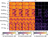 |
Figure 3 Four setups are demonstrated (columns) for each FNO trained (rows). For the multi-source domains this shows time-step t = 40, and for all others this shows t = 72. Multi-source experiments contain between 1 and 4 simultaneous sound sources. Sound source positions are marked in cyan. Scattering and B+S experiments contain a reflective object of a different size. Boundary experiments feature one randomly positioned sound source. Ground-truth and predicted values are converted to decibels with a reference signal strength of unity. (a) Ground-truth FDTD simulations produced using SRL and IWB stencils. (b) FNO predictions: each prediction from an FNO was obtained by providing the early time-steps of simulations pictured in (a) as input data. (c) Absolute difference in decibels between FNO predictions and ground-truth FDTD simulations. |
With this established, superposition was introduced from reflective surfaces, rather than multiple sound sources. Superposition from reflections is modelled more poorly in comparison. Trivial solutions exist for the free-field multiple source experiments, whilst the most complex B+S experiments feature many reflections and diffraction effects. In all examples however, the wavefront is modelled well by the FNO models as they appear darkest in all absolute error plots shown. The most error is apparent around reflective objects, surrounding the opposing faces to where a wave has contacted it.
The FNO is also able to predict the location of reflective objects well in the domain. In the scattering and B+S examples, the silhouettes of the objects can be seen in the absolute error plots, demonstrating that FNO networks predict very little noise inside areas where pressure should equal zero at all times.
Table 4 records the MSE of predictions from all FNO networks trained. These error values represent the MSE of all (x, y, t) points for the examples pictured. FNO models appear to learn more efficiently from FDTD data produced using the SRL stencil function. However, there is very little difference between the errors reported for SRL and IWB configurations, meaning FNO can learn efficiently from both datasets.
MSE values for predictions. Error is quantified over the entire prediction at all grid points. Predictions with the highest error in a set of experiments are highlighted red and those with the lowest error are highlighted in green.
In support of Figure 3c, the amount of error in a prediction scales roughly with problem complexity. This is evident in the error quantified for the multi-source experiments, where error increases with the number of sound sources predicted. Furthermore, all other experiments which introduce reflections report higher MSE values than the reflection-free multi-source tests. This suggests that wave superposition that arises from reflections is harder to model using FNO networks than superposition from multiple sound sources. Incorporating reflective boundaries causes error to rise considerably.
Reflections, and diffraction in the scattering and B+S examples, are more complex phenomena than wave propagation in a free-field with no absorption losses. This produces a more intricate spectra when FDTD data is transformed using the FFT within the FNO hidden layers. In turn, it becomes increasingly difficult for the FNO to map between input and target functional spaces without significantly increasing the volume of training data the model receives. The shape of the reflective object does not appear to affect prediction accuracy meaningfully as the range of values reported is low.
4.1 Frequency-domain analysis
Transfer Functions (TFs) were taken from each domain for analysis and the results are presented in Figure 4. These TFs were obtained by measuring an impulse response from the center point of the grid ((x, y) = (32, 32)). The impulse responses were then transformed using a 4096-point real-valued FFT to plot the magnitude spectra. Transfer functions taken from multi-source predictions agree with ground-truth TFs taken from FDTD simulations well, visible by the similar line plots and by the low MSE values reported. To reinforce previous findings, it can be seen that error in predictions increases with problem complexity.
 |
Figure 4 Transfer functions taken from the center of the domain for SRL and IWB FDTD and FNO solutions. The bold black line marks 1.25 kHz, the cutoff frequency of the lowpass filter that was applied to training data. |
Both the scattering and B+S experiments involve modelling diffraction as the wave is scattered by an object. Diffraction appears to be poorly modelled, as there is often considerable error in the lowest frequency ranges of the TFs for these experiments, where diffraction would be most apparent. This can further be verified by comparing these results to the multi-source and boundary experiments, where the true and predicted TFs match more closely.
As an example, reference the 16 × 16 block result shown in Figures 3a and 3b for the scattering experiment. Strong diffraction effects, caused by the wave glancing from the corner of the block, would be captured by a TF taken from the center of the domain. Consequently, this predicted transfer function shows the greatest deviation from the ground-truth of all.
This suggests that overall MSE reported for domains is skewed by low-valued areas in predictions with fewer sound sources, as previously identified in Figure 3c, and areas with active wave propagation are more strongly affected by FNO error. However, there is still little variance between MSE values reported for TFs taken from scattering and B+S domains, reinforcing the finding that object shape does not significantly affect FNO prediction accuracy.
4.2 Training dynamics
The validation loss curves during training were recorded every epoch and are shown in Figure 5. This data was recorded by evaluating the network at each training epoch on a set of testing data that was not used to adjust network weights. The multi-source experiments converged to the lowest minima and also exhibited the best generalisation out of all the experiments conducted. This confirms the FNO models these relatively simple problems well and can exhibit similar prediction quality whether the input data existed in the training dataset or not. Generalisation immediately suffers once any reflective attributes are introduced to the domain. FNO networks modelling boundary reflections only converged smoothly, demonstrating little instability. In contrast, scattering and B+S models were more unstable, showing large spikes, despite receiving 4200 more FDTD simulation examples in their respective training datasets. This indicates that modelling diffraction is a cause of FNO instability during training given the complexity of the task.
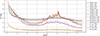 |
Figure 5 FNO network loss values as a function of training epoch. The peak around epoch 50 is caused by the cosine learning rate scheduling function. All FNO networks trained display good generalisation, as evidenced by the similar loss values when evaluated on training and validation data. |
SRL and IWB FNO networks show highly similar trajectories during gradient descent for domains of the same type. This is in agreement with previous observations that FNO can learn from acoustic simulation datasets prepared with SRL and IWB stencils with little meaningful difference between them. FNO networks modelling just boundary reflections converged to the highest values overall. This is due to the difficulty in modelling reflections combined with the low dataset size of 800 FDTD simulations. B+S networks converged to a lower overall minima than scattering networks, despite B+S predictions also reporting higher error. This effect is likely due to the smaller values involved in the scattering experiments as the waves escape past the boundaries in later time-steps, skewing the loss trajectory towards zero.
Figure 6 describes the time taken to train each network, to predict a single solution from the network and how long an equivalent FDTD simulation would take. The time taken to apply the lowpass filter to FDTD data is included in these measurements. FNO prediction times outperform FDTD simulation times by hundreds of milliseconds in all instances. Multi-source FNO networks were the quickest to train as they contain slightly fewer parameters than the others. Multi-source FDTD data was also the fastest to simulate as there are half the number of time-steps involved in the simulation. Boundary and B+S networks were the longest to train as their datasets were  20 GB larger than the other experiments. Despite the fast prediction times, the requirement to train the FNO network for between 1–8 hours makes FNO relatively time-inefficient as a wave-solver when compared to FDTD.

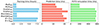 |
Figure 6 FNO training and prediction times, with equivalent FDTD simulation times. |
Equation (9) describes the number of dataset permutations where k is the maximum number of sound sources and A is the area of the reflective object in samples, if present (otherwise A = 0). A complete dataset of FDTD simulations describes a set where each simulation has a unique combination of excitation positions. Given the large factorial values involved, the amount of data required to store a complete dataset in computer memory is unfeasible. As the FNO models demonstrated here have been trained on 800 to 5000 FDTD examples, it can be claimed that the unmodified FNO architecture can learn from compact datasets containing similar problems and generalise to similar problems outside of this dataset.
5 Discussion
Although the FNO network approach to predicting acoustic wave propagation for these relatively simple 2D acoustic problems offers good results when compared to ground-truth FDTD simulations in nearly all examples it is limited in its application as a generally applied efficient solution due to the training time required. However, FNO networks could have a more promising application as a method of data compression for the storage of outputs from the domain (impulse responses). The 24.4 GB training dataset for scattering and B+S domains can be substituted with a 15.5 MB FNO once trained which captures this dataset and generalises to similar examples outside of it. By extension, a complete set of FDTD data with α-many members (Eq. 9) could not be stored on a computer in practice without running out of memory. The on-disk size of the FNO is dictated by the number of parameters rather than the size of the dataset it was trained on. This is useful in situations where a large number of simulations are required for recall in a task; rather than loading pre-simulated FDTD data from computer memory, predictions can be made from the FNO network.
It has been demonstrated that FNO networks can model reflections that arise from boundaries and objects within the domain, further generalising over the shape and position of the object. However, evidence suggests diffraction is captured relatively poorly and is difficult to model using a small dataset. This fact, in conjunction with the relatively unstable loss descents for scattering and B+S experiments in Figure 5, suggests the standard FNO architecture presented here is reaching the limits of its modelling capabilities. Transfer learning [29] could be used to improve generalisation over domain geometry including reflecting objects in the space.
6 Conclusions
This paper has presented FNO networks that are able to generalise over several physical factors while modelling 2D linear acoustic wave propagation in free-field domains. Specifically, FNO networks were able to generalise over arbitrarily positioned excitation sources within the domain, discern the number of excitation sources present in the input data, up to a limit of 4, and learn from two FDTD stencils used in the training data. It was also shown that FNO could solve non-trivial and increasingly difficult problems involving wave superposition caused by reflections from boundaries and rectangular objects, with variable shapes and positions. Evidence suggests that more training data is required to produce high-quality predictions and to ensure FNO stability during training. FNO networks have been shown to predict solutions to the 2D wave equation quickly and consistently, although training the network is a lengthy process and longer in practice than using an equivalent FDTD method.
For larger problem domains in FNO contexts, spatial domain decomposition could be explored using FNO [30]. For typical auralisation use cases where only a single source-receiver pair is required for any one simulation, the FNO becomes inefficient as a lot of unnecessary data is returned when only a single impulse response would suffice. DeepONet [9, 11, 31] methods allow for predictions to be made for a single source-receiver pair, but cannot predict the entire wave-field in one pass. Therefore, it is suggested that FNO is suited towards scenarios where sound pressure level as a function of time over many points in a domain must be evaluated. Future work will conduct auralistion experiments to discern perceptual differences between FNO and FDTD implementations as transfer functions predicted by FNO approximate ground-truth TFs well in many cases, indicating that the FNO should be suitable for signal auralisation purposes.
Funding
This work has been in part sponsored by an Audio Engineering Society Education Foundation Award.
Conflicts of interest
The authors declare that there is no conflict of interest.
Data availability statement
The data and code used in experiments is available from the corresponding author on request.
References
- M. Van Walstijn, K. Kowalczyk: On the numerical solution of the 2D wave equation with compact FDTD schemes, in: Proceedings of the 11th International Conference on Digital Audio Effects, DAFx, 2008, pp. 205–212. [Google Scholar]
- K. Kowalczyk, M. Van Walstijn: Room acoustics simulation using 3D compact explicit FDTD schemes, IEEE Transactions on Audio, Speech, and Language Processing 19, 1 (2011) 34–46. [CrossRef] [Google Scholar]
- C.J. Webb, S. Bilbao: Computing room acoustics with CUDA – 3D FDTD schemes with boundary losses and viscosity, in: 2011 IEEE International Conference on Acoustics, Speech and Signal Processing (ICASSP), 2011, pp. 317–320. [Google Scholar]
- D. Botteldooren: Finite difference time domain simulation of low frequency room acoustic problems, The Journal of the Acoustical Society of America 98, 6 (1995) 3302–3308. [CrossRef] [Google Scholar]
- L. Savioja: Real-time 3D finite-difference time-domain simulation of low and mid-frequency room acoustics, in: DAFX: the 13th International Conference on Digital Audio Effects (DAFx-10), 2010, Graz, Austria. [Google Scholar]
- M. Raissi, P. Perdikaris, G.E. Karniadakis: Physics-informed neural networks: a deep learning framework for solving forward and inverse problems involving nonlinear partial differential equations, Journal of Computational Physics 378 (2019) 686–707. [CrossRef] [Google Scholar]
- Z. Li, N.B. Kovachki, K. Azizzadenesheli, B. Liu, K. Bhattacharya, A.M. Stuart, A. Anandkumar: Fourier neural operator for parametric partial differential equations, in: CoRR abs/2010.08895, 2020. [Google Scholar]
- J.D. Parker, S.J. Schlecht, R. Rabenstein, M. Schäfer: Physical modeling using recurrent neural networks with fast convolutional layers, in: Proceedings of the 25-th International Conference on Digital Audio Effects (DAFx20in22). Ed. by G. Evangelista and N. Holighaus. Vol. 3. Vienna, Austria, Sept. 6–10, 2022, pp. 138–145. [Google Scholar]
- L. Lu, P. Jin, G. Pang, Z. Zhang, G. Karniadakis: Learning nonlinear operators via DeepONet based on the universal approximation theorem of operators, Nature Machine Intelligence 3, 3 (2021) 218–229. [CrossRef] [Google Scholar]
- M. Middleton, D.T Murphy, L. Savioja: The application of Fourier neural operator networks for solving the 2D linear acoustic wave equation, in: Proceedings of the 10th Convention of the European Acoustics Association, Turin, Italy. Forum Acusticum 2023, European Acoustics Association, 2023. [Google Scholar]
- N. Borrel-Jensen, S. Goswami, A. Engsig-Karup, G. Karniadakis, C-H. Jeong: Sound propagation in realistic interactive 3D scenes with parameterized sources using deep neural operators, Proceedings of the National Academy of Sciences 121, 2 (2024) e2312159120. [CrossRef] [PubMed] [Google Scholar]
- K. Kowalczyk, M. Van Walstijn: Wideband and isotropic room acoustics simulation using 2D interpolated FDTD schemes, IEEE Transactions on Audio, Speech, and Language Processing 18, 1 (2010) 78–89. [CrossRef] [Google Scholar]
- H. Kudo, T. Kashiwa, T. Ohtani: The non-standard FDTD method for three-dimensional acoustic analysis and its numerical dispersion and stability condition, Electronics and Communications in Japan (Part III: Fundamental Electronic Science) 85, 9 (2002) 15–24. [CrossRef] [Google Scholar]
- D. Botteldooren: Acoustical finite-difference time-domain simulation in a quasi-Cartesian grid, The Journal of the Acoustical Society of America 95, 5 (1994) 2313–2319. [CrossRef] [Google Scholar]
- L. Savioja, T. Rinne, T. Takala: Simulation of room acoustics with a 3-D finite difference mesh, in: The 1994 International Computer Music Conference, Aarhus, September 12–17, 1994, International Computer Music Association ICMA, United States, 1994, pp. 463–466. [Google Scholar]
- N. Borrel-Jensen, A.P. Engsig-Karup, C-H. Jeong: Physics-informed neural networks for one-dimensional sound field predictions with parameterized sources and impedance boundaries, JASA Express Letters 1, 12 (2021) 122402. [CrossRef] [PubMed] [Google Scholar]
- M. Pezzoli, F. Antonacci, A. Sarti: Implicit neural representation with physics-informed neural networks for the reconstruction of the early part of room impulse responses, in: Proceedings of the 10th Convention of the European Acoustics Association, Turin, Italy. Forum Acusticum 2023, European Acoustics Association, 2023. [Google Scholar]
- T. Zhang, D. Trad, K. Innanen: Learning to solve the elastic wave equation with Fourier neural operators, Geophysics 88, 3 (2023) 101–119. [Google Scholar]
- B. Li, H. Wang, S. Feng, X. Yang, Y. Lin: Solving seismic wave equations on variable velocity models with fourier neural operator, IEEE Transactions on Geoscience and Remote Sensing 61 (2023) 1–18. [CrossRef] [Google Scholar]
- A. Choubineh, J. Chen, D.A. Wood, F. Coenen, F. Ma: Fourier neural operator for fluid flow in small-shape 2D simulated porous media dataset, Algorithms 16, 1 (2023) 24. [CrossRef] [Google Scholar]
- D. Hendrycks, K. Gimpel: Gaussian error linear units (GELUs), 2020. arXiv: 1606.08415 [cs.LG]. [Google Scholar]
- A. Emin Orhan, X. Pitkow: Skip connections eliminate singularities, 2018. arXiv: 1701.09175 [cs.NE]. [Google Scholar]
- L. Lu, X. Meng, S. Cai, Z. Mao, S. Goswami, Z. Zhang, G. Karniadakis: A comprehensive and fair comparison of two neural operators (with practical extensions) based on fair data, Computer Methods in Applied Mechanics and Engineering 393 (2022) 114778. [CrossRef] [Google Scholar]
- G. Wen, Z. Li, K. Azizzadenesheli, A. Anandkumar, S.M. Benson: U-FNO – an enhanced Fourier neural operator-based deep-learning model for multiphase flow, Advances in Water Resources 163 (2022) 104180. [CrossRef] [Google Scholar]
- A. de Cheveigné, I. Nelken: Filters: when, why, and how (not) to use them, Neuron 102, 2 (2019) 280–293. [CrossRef] [PubMed] [Google Scholar]
- A. Koloskova, H. Hendrikx, S.U. Stich: Revisiting gradient clipping: stochastic bias and tight convergence guarantees, in: Proceedings of the 40th International Conference on Machine Learning. Ed. by A. Krause, E. Brunskill, K. Cho, B. Engelhardt, S. Sabato, J. Scarlett, vol. 202. Proceedings of Machine Learning Research. PMLR, 23–29 Jul 2023, pp. 17343–17363. https://proceedings.mlr.press/v202/koloskova23a.html. [Google Scholar]
- W.M. Czarnecki, S. Osindero, M. Jaderberg, G. Åwirszcz, R. Pascanu: Sobolev training for neural networks, 2017. arXiv: 1706.04859 [cs.LG]. [Google Scholar]
- I. Loshchilov, F. Hutter: SGDR: stochastic gradient descent with warm restarts, 2017. arXiv:1608.03983 [cs.LG]. [Google Scholar]
- F. Lehmann, F. Gatti, M. Bertin, D. Clouteau: Seismic hazard analysis with a Fourier neural operator (FNO) surrogate model enhanced by transfer learning, in: NeurIPS AI for Science workshop. New Orleans, United States, Dec. 2023. https://hal.science/hal-04476126. [Google Scholar]
- T.J. Grady, R. Khan, M. Louboutin, Z. Yin, P.A. Witte, R. Chandra, R.J. Hewett, F.J. Herrmann: Model-parallel Fourier neural operators as learned surrogates for large-scale parametric PDEs, Computers and Geosciences 178 (2023) 105402. [CrossRef] [Google Scholar]
- M. Zhu, S. Feng, Y. Lin, L. Lu: Fourier-DeepONet: Fourier-enhanced deep operator networks for full waveform inversion with improved accuracy, generalizability and robustness, Computer Methods in Applied Mechanics and Engineering 416 (2023) 116300. [CrossRef] [Google Scholar]
Cite this article as: Middleton M. Murphy DT. & Savioja L. 2025. Modelling of superposition in 2D linear acoustic wave problems using Fourier neural operator networks. Acta Acustica, 9, 20. https://doi.org/10.1051/aacus/2024078.
All Tables
MSE values for predictions. Error is quantified over the entire prediction at all grid points. Predictions with the highest error in a set of experiments are highlighted red and those with the lowest error are highlighted in green.
All Figures
|
Figure 1 A representation of the FNO network architecture. Layer shapes in tensors are shown in parentheses. The transformed signal is usually truncated with high-frequency FFT bins discarded as a regularisation measure [7]. |
| In the text | |
|
Figure 2 Probability density example for sampling excitation coordinates. 200 coordinates, highlighted in green, are sampled from a B+S domain which contains a 16 × 16 reflective object. Lighter areas have a higher probability of sampling. |
| In the text | |
|
Figure 3 Four setups are demonstrated (columns) for each FNO trained (rows). For the multi-source domains this shows time-step t = 40, and for all others this shows t = 72. Multi-source experiments contain between 1 and 4 simultaneous sound sources. Sound source positions are marked in cyan. Scattering and B+S experiments contain a reflective object of a different size. Boundary experiments feature one randomly positioned sound source. Ground-truth and predicted values are converted to decibels with a reference signal strength of unity. (a) Ground-truth FDTD simulations produced using SRL and IWB stencils. (b) FNO predictions: each prediction from an FNO was obtained by providing the early time-steps of simulations pictured in (a) as input data. (c) Absolute difference in decibels between FNO predictions and ground-truth FDTD simulations. |
| In the text | |
|
Figure 4 Transfer functions taken from the center of the domain for SRL and IWB FDTD and FNO solutions. The bold black line marks 1.25 kHz, the cutoff frequency of the lowpass filter that was applied to training data. |
| In the text | |
|
Figure 5 FNO network loss values as a function of training epoch. The peak around epoch 50 is caused by the cosine learning rate scheduling function. All FNO networks trained display good generalisation, as evidenced by the similar loss values when evaluated on training and validation data. |
| In the text | |
|
Figure 6 FNO training and prediction times, with equivalent FDTD simulation times. |
| In the text | |
Current usage metrics show cumulative count of Article Views (full-text article views including HTML views, PDF and ePub downloads, according to the available data) and Abstracts Views on Vision4Press platform.
Data correspond to usage on the plateform after 2015. The current usage metrics is available 48-96 hours after online publication and is updated daily on week days.
Initial download of the metrics may take a while.