| Issue |
Acta Acust.
Volume 10, 2026
|
|
|---|---|---|
| Article Number | 14 | |
| Number of page(s) | 20 | |
| Section | Hearing, Audiology and Psychoacoustics | |
| DOI | https://doi.org/10.1051/aacus/2026007 | |
| Published online | 06 March 2026 | |
Scientific Article
Evaluation of elevated hearing thresholds produced by models for the simulation of cochlear hearing loss
1
RWTH Aachen University, Institute for Hearing Technology and Acoustics, Kopernikusstraße 5, 52074 Aachen, Germany
2
RWTH Aachen University, Institute of Psychology, Jägerstraße 17-19, 52056 Aachen, Germany
3
RWTH Aachen University, Department of Neurology, Pauwelsstraße 30, 52074 Aachen, Germany
* Corresponding author: This email address is being protected from spambots. You need JavaScript enabled to view it.
Received:
2
August
2025
Accepted:
20
January
2026
Abstract
Introduction: As the statistical distribution of hearing thresholds moves towards stronger hearing impairments with age, plausible simulations of its perceptual effects are useful for a variety of applications. Four software tools for the simulation of hearing loss, capable of generating audible output, were evaluated. An overview of the simulators is presented, their capabilities and significant signal processing steps are introduced. Methods: The perceptual evaluation focuses on the simulation of elevated hearing thresholds. Two listening experiments were conducted to assess how accurately the hearing loss simulators can reproduce target audiograms, i.e., elevated hearing thresholds when normal-hearing listeners are subjected to the simulation. Mild and moderate degrees of simulated hearing loss conditions were defined based on typical hearing thresholds of 70- and 80-year-olds. The complementary technical analysis addresses additional simulated consequences of cochlear hearing loss by investigating input-vs.-output level functions and spectral smearing effects. Results: Statistically significant differences between simulators were found: Good agreement with the target hearing thresholds was found for the simulator “WHIS" (deviations 0 to 6 dB), while the others showed deviations of varying degree (−29 to 7 dB). The created input-output functions proved to be suitable for demonstrating expansive dynamic range processing and explaining the listening experiment results.
Key words: Hearing loss simulation / Hearing model / Auditory modelling / Cochlear model / Audiology
© The Author(s), Published by EDP Sciences, 2026
 This is an Open Access article distributed under the terms of the Creative Commons Attribution License (https://creativecommons.org/licenses/by/4.0), which permits unrestricted use, distribution, and reproduction in any medium, provided the original work is properly cited.
1 Introduction
There are a number of different reasons for realistically, or at least plausibly, simulating hearing loss. For example, raising awareness of hearing loss and its consequences in the public might be regarded as worthwhile, considering the fact that close to 19% of the world population (over 1.5 billion people) were affected by hearing loss in 2021 [1]. With more than 65% of adults older than 60 years experiencing hearing loss, the problem is particularly prevalent among the elderly population. In the context of audio or music production, being able to anticipate how an audio recording will sound for people suffering from hearing loss may be of interest to audio engineers and other content creators, facilitating the assessment and decision as to what extent the audio signal processing needs to be adjusted for this particular group of listeners. Knowledge of how to simulate hearing loss is also relevant when adapting psychoacoustic hearing models to represent the behaviour of an impaired ear, e.g., for calculating loudness, roughness or sharpness values. Furthermore, the successful simulation of hearing loss can be considered useful in the development and assessment of hearing aids and their corresponding signal processing algorithms. Analogously, cochlear implant simulation by vocoder processing has been utilized in research aiming towards the improvement of cochlear implant signal processing algorithms [2, 3]. Hearing loss simulation can be used by researchers as a tool in the context of listening experiments in which normal-hearing participants have their hearing abilities intentionally impaired. Here, a potential goal might be to derive insight into whether differences in performance between young, normal-hearing listeners and elderly listeners with age-related hearing loss can be attributed to sensory deficits, or rather age-related cognitive change.
Due to the complexity of the auditory system, the development of auditory models is no trivial task. The same applies to the development of models for the simulation of hearing loss. Causes of hearing loss are manifold, including genetic factors, infections and other diseases, physical trauma, ototoxic substances, noise-induced hearing loss, and age-related hearing loss. Similarly diverse are the potential symptoms and consequences of hearing loss. This contribution focuses on cochlear hearing loss in particular, since it is considered to be the form of hearing loss encountered most frequently. Even within this limited scope, a variety of possible perceptual consequences are known to exist (for an overview, see [4, 5]) , in particular: increased hearing thresholds, loudness recruitment (i.e., reduced dynamic range), reduced frequency selectivity, and degraded temporal resolution. However, regarding the latter it has been pointed out [4, 5] that the performance deficit in measures of temporal resolution observed for people with cochlear hearing loss can to a large extent be explained by the other well-known consequences of outer hair cell damage: The increased hearing thresholds and the accompanying loudness recruitment lead to lower sensation levels and a narrower effective frequency bandwidth available to the listener, which together with the degraded frequency resolution leads to a decreased amount of neural information available in the following stages of auditory processing and ultimately a decreased efficiency of central decision processes.
The adequate simulation of the aforementioned detrimental effects represents the main goal for the implementation of a corresponding software tool. While solely implementing a simple linear filter which attenuates frequencies according to a desired target hearing threshold might be sufficient for simulating the effect of certain cases of conductive hearing loss, this approach will not suffice to achieve a realistic simulation of cochlear hearing loss, since the human sense of hearing is highly non-linear in nature. For example, in order to let a normal-hearing listener experience the effect of loudness recruitment via simulation, the compressive properties due to the active mechanism of the healthy ear need to be negated to a certain extent (or cancelled out completely for the case of severe outer hair cell loss) by suitable signal processing. The concept is depicted in Figure 1. A digital audio input signal is sent to a processing block of a hearing loss simulator performing inverse compression by implementing an expansive input-output characteristic. This processing happens in anticipation of the compressive properties of the normal-hearing listener’s ear, to whom the processed signal is played back. In combination, the resulting input-output characteristic perceived by the listener is – in the case of severe outer hair cell loss – close to linear, as illustrated in the third block.
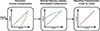 |
Figure 1. Block diagram depicting the input-output characteristics involved in the simulation of loudness recruitment. |
For this contribution, a set of hearing loss simulators with relevant capabilities were gathered from the literature, and a perceptual and technical evaluation was conducted. The following subsection presents an overview of these simulators with a basic explanation of the working principles and features. Two listening experiments based on pure-tone audiometry were conducted with the goal of answering the following research question: How accurately can the simulators produce a predefined audiogram for normal-hearing listeners? By means of one-sample t tests, it is investigated whether there were statistically significant deviations from predefined target hearing thresholds and how large the corresponding effect sizes were. Using repeated-measures analysis of variance, it was assessed whether there were statistically significant differences between the evaluated simulators, and whether there were any interactions with frequency and degree of simulated hearing loss. The accompanying technical evaluation presented in Section 3 focuses on the aspects of elevated hearing thresholds, expansive nonlinearity and altered frequency resolution. The individual simulators covered in this contribution have only been evaluated or validated regarding specific aspects (which vary from case to case) in their corresponding publications. To the authors’ knowledge, no comparably comprehensive and uniform evaluation of multiple hearing loss simulators has been carried out and published thus far. Note that this contribution makes no claim to completeness regarding available hearing loss simulators or potential methods for their analysis and evaluation.
1.1 Evaluated simulators
The selection process and criteria for the simulators ultimately included in the evaluation presented here are outlined in the following. The simulators were expected to be able to create output in the form of an actual audio signal (audio file or real-time stream) intended to be played back to a normal-hearing listener. Not all existing simulation tools are intended for this purpose, such as the “Hearing-Loss Visualizer" [6], which solely visualizes population responses of auditory-nerve fibres and midbrain neurons of hearing-impaired ears. The audible output for the normal-hearing listener should be as realistic, or at least as plausible, as possible. One approach which has been used in the context of hearing loss simulation is the artificial addition of spectrally shaped noise to the original signal. While this method may recreate impaired performance in some specific listening tasks, e.g., as used in the equivalent threshold masking technique to induce elevated hearing thresholds, it is evident that, in general, this does not correspond to what a listener with real hearing loss perceives (cf. [7]). With the possible exception of tinnitus patients, a permanent noise, generated or emerging within the auditory system itself, is not what causes the hearing-impaired listener’s performance deficits. These are the reasons why other methods (i.e., dynamic expansion, level-dependent attenuation) for simulating elevated thresholds and loudness recruitment were preferred for the evaluation presented here. For an assessment of the equivalent threshold masking technique, see [8]. Particularly for the potential use in listening experiments, the possibility of entering a predetermined target audiogram (i.e., the hearing threshold as a function of frequency) was defined as an essential feature. The availability of a dedicated publication about the simulator, or at least about the software suite or project of which it may be a part, was deemed preferable. A dedicated website and any other form of existing documentation were considered beneficial as well. The use of the simulator in published studies or projects was also taken into account for the selection. Finally, accessibility and applicability for a wide range of users were also considered relevant. Potentially suitable simulators were found via a combination of online-search results, personal exchange with researchers working in related fields, and prominent use in published studies or projects.
The following subsections introduce the hearing loss simulators that were evaluated; Table 1 provides an overview. This will include an outline of their main features, model structure, and basic signal processing steps. To conclude the introduction, we would like to draw the reader’s attention to a number of additional examples of simulation software, which, while not forming part of the present evaluation, are worthy of consideration.
Overview of the hearing loss simulators considered for evaluation in the context of this study, specifying the programming language they are implemented in, whether they are openly available online, whether the signal processing can be achieved in real-time, and whether they can be operated via a graphical user interface (GUI).
While it is not the main focus of this software toolbox and framework, a hearing loss simulation is included in the “open Master Hearing Aid (openMHA)”, developed in the context of the “open community platform for hearing aid algorithm research" project [9]. By the time of the commit of the corresponding code to the project’s Github repository [10], May 2024, the listening experiments presented in this contribution had already been completed.
For their study of efferent reflexes in the encoding of speech by the auditory nerve, Grange et al. [11] developed a model named “MAPsim”, based on the physiological “MATLAB Auditory Periphery (MAP)" model of Meddis et al. [12]. Within the MAP model, it is possible to manipulate or deactivate individual components of the auditory system. Grange et al. expanded the MAP model by a decoder module which reconstructs an audible signal from the auditory nerve output of the MAP encoder, including the implemented experimental impairments or manipulations. Using MAPsim, the configuration of a target audiogram is more complex than for the simulators selected for our evaluation. The use of MAPsim requires more in-depth knowledge of the physiological mechanisms underlying the auditory pathway, as many physiology-related parameters need to be configured. Grange et al. note that the code for their MAPsim model is available on request.
For their study of emotion recognition with impaired vision and hearing, a hearing impairment simulation was implemented by de Boer et al. [13]. Additional description of this simulator can be found in Jürgens et al. [14], where it was used to investigate spatial speech-in-noise performance of normal-hearing listeners with simulated single-sided deafness and bimodal cochlear implant use. Their hearing impairment simulator is based on the “Cambridge Hearing Loss Simulator”, the details of which are presented in Section 1.1.1.
Finally, the hearing loss simulator by Grimault et al. [7] was originally part of this study, but due to a user error made in the context of the calibration of the stimuli for this simulator, the corresponding results were omitted and are therefore not presented or discussed in the following.
1.1.1 Clarity / Cambridge Hearing Loss Simulator
The Clarity project was initiated with the goal of improving speech-in-noise signal processing algorithms of hearing aids [15]. For this purpose, the project provides open-source material [16] such as models for hearing aid processing, including testing and training data. Also included is a model for the simulation of hearing impairment; this simulator is a reimplementation of the Cambridge Hearing Loss Simulator (CHLS) in Python. The main contributors to the implementation and the theory behind the CHLS are Thomas Baer, Brian Moore, Brian Glasberg, Yoshito Nejime, and Michael Stone [17–21]. It has been used, e.g., in the context of investigating the effects of age-related hearing loss on speech perception using automatic speech recognition [22]. The simulator was originally implemented as a collection of MATLAB (MathWorks, Natick, Massachusetts, United States) files and (in older versions) C executables. Due to the advantages of an implementation in Python (free and open source), combined with its accessibility and documentation on a GitHub repository, the Clarity project’s implementation of this simulator was selected for the evaluation presented here. Its basic signal processing steps are shown in the block diagram of Figure 2.
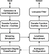 |
Figure 2. Block diagram of the processing steps of the Clarity / Cambridge Hearing Loss Simulator. |
The initial configuration of the simulator comprises the definition of a target audiogram: Hearing level values for 15 frequencies ranging from 125 Hz to 16 kHz are entered. As a first step in the processing, the user enters the root mean square (RMS) sound pressure level which the source signal (a digital audio file) is supposed to have. Next, a transfer function is applied (linear filtering), describing the assumed influence of the transfer path from the sound source to the cochlea. Available options for the transfer function are “free field" (frontal incidence), “diffuse field”, and “ITU”, the latter referring to ITU recommendation P.58 [23]. The actual hearing loss simulation itself is carried out in two main processing steps. First, the “spectral smearing" aims to simulate the reduced frequency resolution of the hearing-impaired listener. Details of the method are described in [17, 18]. For each centre frequency, the amount of spectral smearing is determined by the audiometric threshold at that frequency. The spectral smearing is followed by the loudness recruitment simulation, which again considers the configuration of audiometric thresholds at the different frequencies. This method is presented in more detail in [19, 21]. After the recruitment simulation, the signal is filtered by employing a transfer function (cochlea-to-source) inverse to the source-to-cochlea transfer function used before the spectral smearing. Finally, a low-pass filter at the end of the signal chain is utilized to prevent uncontrolled behaviour at high frequencies, since audiogram data can only be entered up to a frequency of 16 kHz. By default, its cutoff frequency is set to 18 kHz.
1.1.2 Wadai hearing impairment simulator
The Wadai Hearing Impairment Simulator (WHIS) was developed at Wakayama University and implemented in MATLAB, refer to [24] for online information. For our evaluation, version 300 of the simulator was used. An updated version has since been released [25]. A series of publications describes the development of its components and examples of application [26–31]. The block diagram in Figure 3 shows the basic processing steps involved.
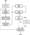 |
Figure 3. Block diagram of the processing steps of the Wadai Hearing Impairment Simulator (WHIS). |
Via the graphical user interface, the user is able to define a target hearing loss (i.e., hearing levels) at seven frequencies ranging from 125 Hz to 8 kHz. Additionally, the parameter “compression health”, which refers to the percentage of healthy outer hair cells, has to be set for each of these frequencies. As a first step, a calibration process has to be completed, establishing the relation between digital levels and sound pressure levels. Before the intended output signal can be generated, the input signal needs to be passed through a series of analysis steps. The signal is first processed with an equalization function based on the work of Meddis [32], which is supposed to model the transition from mechanical vibrations of the basilar membrane to action potentials originating from the inner hair cells. Similar to the Clarity simulator, the signal is processed using a transfer function which describes the transfer path from the sound source to the cochlea (again, options such as “free field" or “diffuse field" are available). The signal is then processed by the “gammachirp" filterbank, which represents a further development of the well-known gammatone filterbank, produced by gammatone filters in combination with a low-pass asymmetric function. Together with a version of the signal processed with an additional high-pass asymmetric function (HP-AF), a level estimation is carried out. The result of this step is fed to an input-output function modelling the contribution of the outer hair cell (OHC) loss to the target total hearing loss defined by the user. From this knowledge, the corresponding contribution of the inner hair cell (IHC) loss is derived. Finally, the calibrated input signal is processed by the “direct time varying filter”, which splits the signal into time frames using a Hanning window and applies non-linear time-varying filtering based on the analysis part of the model.
1.1.3 3D Tune-In toolkit
This open-source toolkit [33] was developed in the context of the 3D Tune-In (3DTI) project [34] and encompasses means for audio spatialization as well as the simulation of hearing loss and hearing aids. Its content has been presented in a number of publications [35–37] and was made available in three different versions: a C++ library, which offers the greatest flexibility, the Binaural Test Application, which combines most of the toolkit’s features in the form of a desktop application, and a VST-plugin suite, where the different components of the toolkit can be loaded and used separately (e.g., the hearing loss simulator on its own). Figure 4 shows an overview of the signal processing steps of the hearing loss simulator.
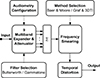 |
Figure 4. Block diagram of the processing steps of the hearing loss simulator included as part of the 3DTI toolkit. |
Regarding the calibration, a static relation between digital levels and sound pressure levels is used: A digital signal level of 0 dB FS is interpreted as corresponding to 100 dB SPL. Thus, the user needs to scale the amplitude of the input audio material appropriately before sending it through the simulator. Similar to the Clarity simulator, the user initially defines audiogram data, i.e., hearing levels at nine frequencies ranging from 62.5 Hz to 16 kHz. The first step of the signal processing consists of a filterbank, which, depending on the selection, splits the input signal either into 27 1/3-octave bands using second-order Butterworth filters or into 42 bands using gammatone filters. These frequency bands are subsequently grouped into nine bands, each corresponding to an octave. These octave bands are then each sent through a separate expander and associated attenuator. While all settings could theoretically be configured manually, several settings of the multiband expander and attenuation block (i.e., threshold, ratio, attenuation) can be configured automatically based on the user-defined hearing levels by choosing the so-called “3DTI model”, which was based on the work of Rasetshwane et al. [38]. In the case of the VST-plugin, there is no manual option and the 3DTI model has to be used. After expansion and attenuation, the frequency bands are combined, and the signal is passed on to the “frequency smearing" block. Two methods for frequency smearing are available: “Baer & Moore" and “Graf+3DTI". The former option refers to the method described by Baer & Moore [17] – the same as was used in the Cambridge Hearing Loss Simulator – while the latter option was implemented based on the work of Badri, Siegel, & Wright [39]. For both smearing methods, presets “none”, “mild”, “moderate”, and “severe" are available. Finally, the signal is processed by the “temporal distortion" block, which aims to mimic the consequences of age-related impairments of neural synchronization in the midbrain [40, 41]. The signal is first split into two frequency bands: While the upper frequency band remains unaffected (with the exception of a compensation delay), a jitter generator introduces random sample displacements into the lower frequency band before the two bands are recombined. The user can specify the crossover frequency as well as the standard deviation, the bandwidth, and the autocorrelation of the white Gaussian noise used for the random process. Moreover, the correlation of the jitter noise between the left and right channels can be controlled when linked processing for the two ears has been enabled. Similar to the frequency smearing, presets for “none”, “mild”, “moderate”, and “severe" are available.
1.1.4 Mourgela et al.
The hearing loss simulator of Mourgela et al. [42] was developed at Queen Mary University of London with the main intention of providing a tool to facilitate listening with simulated hearing loss in the context of working with digital audio workstation (DAW) software. It was implemented as a VST-plugin and is thus real-time capable. The block diagram in Figure 5 shows the basic processing steps for one of the two input channels, which can be configured independently.
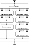 |
Figure 5. Block diagram of the processing steps of the hearing loss simulator of Mourgela et al. |
First, the input signal is sent through a gammatone filterbank and split into 32 frequency bands with equal spacing on the equivalent rectangular bandwidth (ERB) scale over the range 20 Hz to 16 kHz. These 32 bands are split into one branch of processing for the lower 11 bands (up to a centre frequency of 729 Hz) and a second branch for the upper 21 bands. The lower frequency bands are combined and processed with the “temporal disruption" block. This processing step introduces temporal jitter into the signal and aims to simulate an impaired listener’s reduced temporal resolution. For this purpose, random phase shifts between −π/2 and 0 are added to the signal phase in the frequency domain. The first processing step for the higher frequency branch is the “spectral smearing”, with the goal of simulating reduced frequency resolution. This is realized by first generating white noise from normally distributed random numbers. Depending on whether the “low" or “high" setting for the intensity of the smearing is chosen (“bypass”, i.e., deactivating the block, is an option as well), this noise is subsequently low-pass filtered with a cutoff frequency of 100 Hz or 200 Hz. The resulting filtered white noise is multiplied with the content of the high frequency bands. For the frequency spectrum of a pure-tone input signal, for example, this results in a noise-like plateau surrounding the frequency of the input tone (see Sect. 3.2 for examples). As a next step, frequency-dependent attenuation is applied by means of a multiband parametric equalizer, which constitutes the most important processing step in realizing simulated elevated hearing thresholds. Presets for a “mild" and a “moderate" hearing loss are available. The last processing step in the high-frequency branch is the “rapid loudness growth" function, which is included to simulate the effect of loudness recruitment. This is realized by sending each frequency band through a separate expander, configured for a threshold of −50 dB FS but returning to a linear “input = output" behaviour above a level of −20 dB FS. Finally, all high frequency bands and the one low frequency band are combined. Neither the VST-plugin nor the corresponding MATLAB code provide a means to calibrate the system, i.e., establish a relation between digital levels and sound pressure levels.
2 Perceptual evaluation
2.1 Audiometry system and signals
At the Institute for Hearing Technology and Acoustics (IHTA), commercial audiometry systems of type “ear3.0" (AURITEC, Hamburg, Germany), used in conjunction with “HDA 300" (Sennheiser, Wedemark, Germany) audiometric headphones are available. But these systems do not allow access to or manipulation of the audiometric test signals (such as sending these signals through hearing loss simulation software). Since exactly such a capability was needed for the planned experiments, a custom-made (software) solution was implemented in MATLAB, based on the same hardware (i.e., the ear3.0 audio interface and the HDA 300 headphones). For this purpose, the audiometric signals, i.e., the pulsed pure tones, generated by the ear3.0 system were recreated. Measurements of sound pressure levels were done using an “Artificial Ear Type 4153" (Brüel & Kjær (B&K), Nærum, Denmark) with a B&K “4192" microphone, connected to a microphone preamplifier B&K “2669" and conditioning amplifier B&K “Nexus Type 2691”, and recorded via an audio interface (RME “Fireface UC”, Audio AG, Haimhausen, Germany). To ensure equality of the ear3.0 and the newly created signals, electric measurements were carried out as well. As shown in Figure 6, the resulting signal temporal envelope is compliant with the requirements for automatic pulsed presentation of sinusoidal tones defined by standard DIN EN 60645-1 [43]. To assess potential spectral splatter caused by the rising and the falling edge of the temporal envelope, auditory spectrograms were created using the Auditory Modeling Toolbox, version 1.6 [44]. Figure 7 shows the result for a pulsed tone with a carrier frequency of 1 kHz, covering the same time span as depicted in Figure 6. The auditory spectrograms revealed no signs of pronounced spectral splatter.
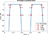 |
Figure 6. Implemented temporal envelope of the pulsed tones. Time constants t BC = 21 ms, t EG = 21 ms, t CE = 222 ms, t FJ = 261 ms, t JK = 239 ms meet the requirements defined in DIN EN 60645-1 [43]. |
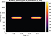 |
Figure 7. Auditory spectrogram of the pulsed tone signal with a carrier frequency of 1 kHz. |
In addition to the technical evaluation of the audiometric signals, a validation experiment was conducted in order to ensure that the results (i.e., hearing thresholds) obtained with the newly created system were close to the ones obtained using the AURITEC system. The participants of Experiment 2 (N = 20, normal-hearing, 5 female, 15 male, see Sect. 2.5.2) completed the experiment. Every participant completed two pure-tone audiometries: Participants with odd-numbered IDs started with the newly developed system, while participants with even-numbered IDs started with the AURITEC system. Both systems were configured to use a step size for the hearing level control of 3 dB. Each software was controlled manually by the tester. For the results shown in the boxplot of Figure 8, the hearing thresholds measured with the AURITEC system were subtracted from the thresholds obtained using the newly developed system. The mean differences between the two systems were between −0.3 s and 2.1 dB for the range of audiometric frequencies shown, with an overall mean difference of 1.3 dB. There was a slight tendency for a larger spread of results towards higher frequencies. This is consistent with the known increase of measurement uncertainty for higher frequencies for pure-tone audiometry, as described in ISO 8253-1 [45].
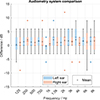 |
Figure 8. Boxplot showing the differences between the hearing thresholds measured using the two audiometry systems. |
2.2 Experimental design
The main goal of the perceptual evaluation was to assess how accurately the simulators can produce a predefined audiogram result for normal-hearing listeners. The independent variables were simulator, frequency, and degree of hearing loss (mild and moderate). The target hearing thresholds for the simulation were chosen to be representative of 70-year-olds (mild condition) and 80-year-olds (moderate condition), as these represent conditions with a high prevalence among the population. The specific hearing threshold values were defined based on data provided by ISO 7029 [46], which gives the statistical distribution of hearing thresholds related to age and gender. For a given frequency and age group, the median hearing thresholds for women and men were averaged. The resulting values were rounded to the nearest multiple of 5 to facilitate the interpretation of the experiment results. This simplification seemed reasonable, given the limited measurement precision of the pure-tone audiometry method (refer to Sect. 4 for further details). Table 2 shows the tested audiometric frequencies and the corresponding target hearing thresholds.
Tested audiometric frequencies and corresponding target hearing thresholds (dB HL) for experimental conditions mild and moderate.
Experiments 1 and 2 shared a common experimental design and the hardware involved, while they differed in the participant group, the set of evaluated simulators and the test environment. All conditions were presented in a counterbalanced order based on a uniformly distributed random Latin square design [47] and tested with both ears. The simulators were evaluated in two separate experiments for two reasons: (1) acquisition and preparation were not completed at the same time for all simulators, and (2) the duration of a single experiment was not supposed to exceed 90 min per participant.
2.3 Configuration of simulators
The defined target hearing thresholds according to Table 2 were entered into the simulators via their respective means (source code or GUI). Where possible, the calibration was configured to correspond to the intended sound pressure levels of the audiometric signals. The WHIS requires the definition of the parameter “compression health”, which is linked to the percentage of remaining healthy outer hair cells. The values used for the simulation were based on findings by Wu et al. [48]. Their study investigated neural degeneration including outer hair cell loss in human cochleas. Outer hair cell survival rates for the two elderly age groups presented were found to be approximately 55% and 35% (see [48], p. 4443); these values were used as a basis for the compression health configuration. Since the WHIS assumes the target hearing loss to result from a combination of inner and outer hair cell loss, the simulator carries out a feasibility calculation after the user enters compression health values as part of the configuration, determining whether the specified target hearing levels can be reached using the given values. This was not the case for several of the audiometric frequencies, with the consequence that the simulator automatically readjusted the compression health to the minimum values deemed valid. The compression health values used are shown in Table 3.
Compression health (CH) values used for the configuration of the WHIS.
For the 3DTI simulator, the stimuli were generated using its VST-plugin version, loaded into the DAW software “Cubase 10" (Steinberg Media Technologies, Hamburg, Germany). During preliminary testing, it was observed that the use of the filterbank option “Gammatone" added an unnatural quality to the sound, which is why the “Butterworth" option was selected for the generation of the final stimuli. Since the 3DTI simulator provides two different methods for frequency smearing (“Baer & Moore" and “Graf+3DTI"), two versions of the stimuli were created for the evaluation of this simulator, each using one of the two methods. For the mild and moderate conditions, the frequency smearing presets labelled “mild" and “moderate" were selected, respectively. For the stimuli included in the experiments, the goal was to simulate the sensory (specifically, cochlear) components of typically encountered age-related hearing loss, rather than any potential neurological components. Thus, the optional “temporal distortion" block of the 3DTI simulator, intended to simulate consequences of age-related impairments of neural synchronization in the midbrain, was deactivated for the generation of the stimuli. For the simulator of Mourgela et al., the attenuation values of the parametric equalizer filterbank were adjusted in such a way that the combined transfer function of the equalizer bands matched the target hearing loss at the tested audiometric frequencies. After completion of the setup, all prepared audiometric signals (i.e., pulsed tones for all frequencies and all hearing levels) were sent through the simulators to be processed accordingly and yield the stimuli for the perceptual and further technical evaluation. Signals for the simulators WHIS and Mourgela et al. were exported with a step size of 5 dB, starting from a hearing level of −10 dB HL, while signals for the simulators 3DTI and Clarity were exported with a step size of 3 dB, starting from −9 dB HL.
2.4 Experiment 1
In the case of Experiment 1, the set of evaluated simulators comprised the simulators WHIS, Mourgela, and Grimault (the results of which were later omitted, as explained in Sect. 1.1).
2.4.1 Experiment 1 – Procedure
After the initial instruction, participants first completed a regular pure-tone audiometry (without hearing loss simulation). This initial audiometry served two purposes: First, verifying whether the participant had normal hearing, and second, providing the actual individual hearing threshold values to be considered in post-processing of the results. Subsequently, participants completed the main part of the experiment, consisting of six (3 simulators × 2 degrees of hearing loss) audiometries including hearing loss simulation. The experiment was conducted in an anechoic chamber at IHTA. Completion took roughly 70–80 min per participant, including short breaks.
2.4.2 Experiment 1 – Participants
Twenty-two participants (12 female, 10 male) completed the experiment. All had normal hearing (hearing threshold < 20 dB HL for all tested audiometric frequencies in the range 125 Hz to 8 kHz). The mean age was 24 years (age range 20–27 years). Participants were volunteers and provided written informed consent to take part in the study. All personal data and experimental results were collected, processed and stored in accordance with German data protection regulations. The Ethics Committee of the Faculty of Medicine, RWTH Aachen University, waived the need for ethics approval for this non-invasive study with healthy, adult participants.
2.4.3 Experiment 1 – Results
As expected, the participants showed individual deviations from the “ideal" hearing threshold of 0 dB HL. To account for these deviations, individual hearing thresholds were subtracted from the corresponding results (same frequency and ear) for the simulated hearing loss conditions. As the results for the left and right ears were highly similar, mean values for the left and right ears are presented hereafter.
The boxplots of Figures 9 and 10 show the hearing thresholds for the mild and moderate hearing loss conditions, respectively, along with the corresponding target values. The mean deviations from the target values are shown in Figures 11 and 12 for the mild and moderate conditions, respectively. For the Mourgela simulator, the results for the mild condition were close to the target values, the largest deviation being −7dB at 8 kHz. The deviations were generally larger for this simulator for the moderate condition: Thresholds were too low for the lower frequencies 125 to 500 Hz and most notably for 8 kHz, which shows a mean deviation of −16 dB. The results for the WHIS simulator were in good agreement with the target values. For the mild condition, the maximum deviation was about 5 dB above target at 125 Hz and 8 kHz, while deviations were 3.5 dB or less for the other frequencies. For the moderate condition, the measured median values exactly matched the target value for four out of the seven audiometric frequencies, while deviations for the remaining three frequencies were between 2 and 5.8 dB.
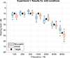 |
Figure 9. Experiment 1: Boxplot showing the hearing threshold results for the mild hearing loss condition. |
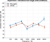 |
Figure 10. Experiment 1: Boxplot showing the hearing threshold results for the moderate hearing loss condition. |
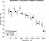 |
Figure 11. Experiment 1: Mean deviations from the target hearing thresholds for the mild hearing loss condition. Error bars show the 95% CI. |
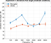 |
Figure 12. Experiment 1: Mean deviations from the target hearing thresholds for the moderate hearing loss condition. Error bars show the 95% CI. |
The statistical analyses described hereafter were conducted using the JASP 0.18.3 software [49].
To investigate whether the observed deviations from the predefined target thresholds were statistically significant, one-sample t tests were conducted. For these tests, the predefined value μ 0 was set to 0 dB (i.e., no deviation from the target threshold). To achieve an acceptable balance between the risk of type I errors and the risk of type II errors, the significance level was moderately adjusted to α = 0.01, while not using a correction for multiple testing.
The results are shown in Table , including effect size and Bayes factor BF01. Overall, the results are consistent with the descriptive statistics. For the Mourgela simulator, only the frequencies 250 Hz and 4 kHz did not show significant deviations from the target for the mild condition. For the moderate condition, no significant deviations were found only for frequencies 1, 2, and 4 kHz. For the WHIS simulator and the mild condition, no significant deviations were found only for frequencies 500 Hz, 2 kHz, and 4 kHz. For the case of the moderate conditions, the null hypothesis was rejected for frequencies 125 Hz, 250 Hz, and 1 kHz.
A three-way repeated measures analysis of variance (RM ANOVA) was conducted with the independent variables simulator, degree of hearing loss, and frequency. The significance level was chosen to be α = 0.05. In cases where Mauchly’s test of sphericity indicated that the assumption of sphericity was violated (p < 0.05), the Greenhouse-Geisser (GG) correction was used for ε(GG)< 0.75, while the Huynh-Feldt (HF) correction was chosen in cases of ε(GG)> 0.75. The results are shown in Table . The effect of simulator was significant, F(1, 20)=119.08, p < 0.001, partial η 2 = 0.86. There were significant effects of degree of hearing loss, F(1, 20)=261.74, p < 0.001, partial η 2 = 0.929, and frequency, F(3.303, 66.053)=30.92, p < 0.001, partial η 2 = 0.61, ε(GG)=0.55. All three main effects can be considered large. All interaction effects were significant: Simulator × Degree of hearing loss: F(1, 20)=172.73, p < 0.001, partial η 2 = 0.9, Simulator × Frequency: F(3.239, 64.783)=91.67, p < 0.001, partial η 2 = 0.82, ε(GG)=0.54, Degree of hearing loss × Frequency: F(3.946, 78.929)=26.78, p < 0.001, partial η 2 = 0.57, ε(GG)=0.658, Simulator × Degree of hearing loss × Frequency: F(2.682, 53.634)=19.68, p < 0.001, partial η 2 = 0.5, ε(GG)=0.447. Differences between simulators Mourgela and WHIS were influenced by the degree of hearing loss especially for lower frequencies. Again, the observed effect sizes can be considered large.
2.5 Experiment 2
In Experiment 2, the simulators Clarity and 3DTI were evaluated, the latter in its two versions due to the different frequency smearing settings: Baer&Moore and Graf&3DTI. Based on the experience gained from Experiment 1, the step size for the hearing level control was reduced from 5 dB to 3 dB to increase measurement accuracy.
2.5.1 Experiment 2 – Procedure
Unlike Experiment 1, Experiment 2 started with two regular audiometric tests: one using the ear3.0 software by AURITEC, the other using the newly developed software, for the purpose of comparing these two audiometry systems, as described in Section 2.1. This was followed by the main experiment, consisting of six (3 simulators × 2 degrees of hearing loss) audiometries including hearing loss simulation. In the case of this experiment, participants were seated in an isolated hearing booth at IHTA. The total duration including breaks was roughly 70–80 min per participant.
2.5.2 Experiment 2 – Participants
Twenty participants (5 female, 15 male) completed the experiment. All had normal hearing (hearing threshold < 20 dB HL for all tested audiometric frequencies in the range 125 Hz to 8 kHz), with a mean age of 26 years (age range 22–41 years). Participants were volunteers and provided written informed consent to take part in the study. All personal data and experimental results were collected, processed and stored in accordance with German data protection regulations. The Ethics Committee of the Faculty of Medicine, RWTH Aachen University, waived the need for ethics approval for this non-invasive study with healthy, adult participants.
2.5.3 Experiment 2 – Results
The post-processing steps were identical to those for Experiment 1.
The boxplots of Figures 13 and 14 show the results for the mild and moderate hearing loss conditions, respectively. Figure 15 (mild condition) and Figure 16 (moderate condition) show the corresponding deviations from the target values. The results for the two frequency smearing methods (Baer&Moore and Graf&3DTI) of the simulator 3DTI, were highly similar, with either identical median values or differences not exceeding 3 dB. This held for both the mild and the moderate condition. The hearing threshold values for the 3DTI simulator were generally lower than the target values. For the mild condition, the thresholds were fairly close to the targets for frequencies up to 2 kHz, about 8 dB too low at 4 kHz, and around 20 dB too low at 8 kHz. For the moderate condition, the thresholds were fairly accurate up to 2 kHz, but around 10 dB too low at 4 kHz and 30 dB too low at 8 kHz. For the Clarity simulator, the hearing thresholds tended to be slightly too high (3 to 7 dB) for frequencies up to and including 4 kHz, while being too low at 8 kHz, deviating by −6 and −9dB for the mild and the moderate conditions, respectively.
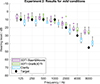 |
Figure 13. Experiment 2: Boxplot showing the hearing threshold results for the mild hearing loss condition. |
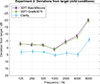 |
Figure 14. Experiment 2: Boxplot showing the hearing threshold results for the moderate hearing loss condition. |
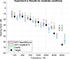 |
Figure 15. Experiment 2: Mean deviations from the target hearing thresholds for the mild hearing loss condition. Error bars show the 95% CI. |
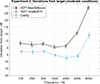 |
Figure 16. Experiment 2: Mean deviations from the target hearing thresholds for the moderate hearing loss condition. Error bars show the 95% CI. |
The results of one-sample t tests can be found in Table . Results for the two variants of the 3DTI simulator (Baer&Moore and Graf&3DTI) were very similar: In both cases for the mild condition, 1 kHz was the only frequency for which no significant deviation was found. For the moderate condition, both variants showed no significant deviations only at 1 and 2 kHz. For the Clarity simulator, the deviations for all frequencies were significant, for both the mild and moderate conditions.
A three-way RM ANOVA was conducted, with independent variables simulator, degree of hearing loss, and frequency. Table shows the results. The main effects of all three independent variables were significant: For simulator: F(2, 38)=2301.61, p < 0.001, partial η 2 = 0.99, for degree of hearing loss: F(1, 19)=60.54, p < 0.001, partial η 2 = 0.76, and frequency: F(3.92, 74.52)=318.84, p < 0.001, partial η 2 = 0.94, ε(GG)=0.65. All three main effects can be considered large. All interactions were again significant and showed large effect sizes: Simulator × Degree of hearing loss: F(2, 38)=25.89, p < 0.001, partial η 2 = 0.58, Simulator × Frequency: F(5.25, 99.82)=151.28, p < 0.001, partial η 2 = 0.89, ε(GG)=0.44, Degree of hearing loss × Frequency: F(6, 114)=117.57, p < 0.001, partial η 2 = 0.86, Simulator × Degree of hearing loss × Frequency: F(6.45, 122.52)=8.82, p < 0.001, partial η 2 = 0.32, ε(GG)=0.54. The two-way interactions were dominated by the increasing difference between the simulators at higher frequencies, while the effect of the three-way interaction was less pronounced than for Experiment 1.
Since the results for the two 3DTI simulator variants were highly similar, a separate RM ANOVA was conducted which only included these two 3DTI variants (i.e., excluding the Clarity simulator results). The observed similarity was corroborated: No significant main effect for simulator remained, F(1, 19)=2.5, p = 0.131, partial η 2 = 0.12. The interactions of Simulator × Degree of hearing loss, F(1, 19)=1.49, p = 0.237, partial η 2 = 0.07, and Simulator × Frequency, F(3.88, 73.67)=0.72, p = 0.579, partial η 2 = 0.04, ε(GG)=0.65, were also no longer significant.
3 Technical evaluation
3.1 Input-output functions
In order to demonstrate and assess the recruitment simulation, and to explain the perceptual results, input-output functions were created for every simulator. For this purpose, the RMS level of each audiometric signal (described in Sect. 2.1), after sending it through the processing of a simulator with a given configuration, was calculated. Figures 17 and 18 show the results for the mild and the moderate hearing loss configurations, respectively; plotted are output hearing levels as a function of input hearing level of the audiometric stimuli. The resulting lines represent a linear interpolation between individual data points. Input-output functions based on peak levels were created as well but proved to be highly similar to the ones based on RMS levels, which is why only the latter version is presented here. In the diagrams, the grey dashed line represents a reference for a linear “input = output" behaviour without any form of amplification or attenuation of the input signal. The area of likely inaudible stimuli (negative output hearing levels) is shaded in grey. A linear filtering, e.g., by simply employing a low-pass filter or equalizer for attenuation, would result in a line with a slope of 1, below and parallel to the reference line. For the simulation of loudness recruitment, the resulting line (or curve) should show attenuated output especially for lower input levels, while gradually coming closer to the reference line for higher input levels. It will at least at some point need to exhibit a slope greater than 1. For explaining the results of the perceptual experiments, the x-intercepts of the result lines, i.e., the input hearing levels at which 0 dB HL output hearing level is exceeded, are particularly relevant. For input hearing levels which are equal to the target threshold, the corresponding output hearing levels should ideally be 0 dB HL.
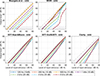 |
Figure 17. Input-output functions, i.e., output hearing levels as a function of input hearing level of the audiometric stimuli, for the simulators configured for the mild degree of hearing loss (target hearing thresholds for the different frequencies provided in parentheses). |
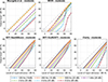 |
Figure 18. Input-output functions, i.e., output hearing levels as a function of input hearing level of the audiometric stimuli, for the simulators configured for the moderate degree of hearing loss (target hearing thresholds for the different frequencies provided in parentheses). |
The simulators exhibited distinctly different behaviour. Slopes with uniform steepness occurred (in the case of the Clarity simulator), while for the other simulators, the slopes changed gradually (3DTI simulator) or more abruptly (WHIS simulator). The input-output functions observed for the WHIS simulator are approximately the inverse of known cochlear compression behaviour. The Mourgela simulator seemingly behaves like a linear system, showing a slope of 1, i.e., a constant attenuation, for each frequency over the range of input signal levels – the only exception being the transition from 75 dB HL to the highest input level of 80 dB HL for the mild condition. While the digital levels of the audiometric input signals used for the analysis covered both the range below the expander threshold of −50dB FS and the range above it, the non-linear processing expected from the “rapid loudness growth” (expansive input-output) function is not visible in this scenario, i.e., the combination of the pulsed pure tones and the expander attack time of 0.3 s and release time of 0.2 s.
The results for the two different frequency smearing methods Baer&Moore and Graf&3DTI of the 3DTI simulator were almost identical – for both degrees of hearing loss, for all frequencies, and for all input levels, with differences < 0.1 dB in many cases.
For many of the combinations of simulator, frequency, and degree of hearing loss, the x-intercepts are in good agreement with the perceptual results of Experiments 1 and 2. In particular, these values predict the good performance of the WHIS simulator, the highly similar results for the two frequency smearing methods of the 3DTI simulator, and the lower-than-target hearing levels at 8 kHz in the case of the Mourgela, 3DTI (Baer&Moore), 3DTI (Graf&3DTI), and Clarity simulators.
The results for the WHIS simulator at 8 kHz in the moderate condition represent an interesting case: While the x-intercept predicts a hearing threshold of about 62 dB HL, and the median value of the perceptual results exactly matches the target hearing level of 65 dB HL, the output level for 65 dB HL input level is actually about 13.6 dB HL, i.e., 13.6 dB higher than what should ideally be found.
When reducing the input hearing level from higher to lower levels, the exact behaviour of a simulator is likely irrelevant once the output level has dropped below 0 dB HL. In this region, a further reduction of the input hearing level will likely cause the output to become and remain inaudible. This would only not apply in the event that the simulator underwent a sudden and drastic change in its level-dependent behaviour at very low input levels. However, such behaviour was not observed in any of the simulators evaluated here.
3.2 Spectral analysis
To assess the effect of frequency smearing (or other steps potentially broadening the frequency spectrum) on the audiometric signals used in the evaluation, a single cycle of the temporal envelope of the pulsed pure-tone signal, as shown in the left half of Figure 6, was Fourier transformed. The duration of the transformed signal excerpt was 500 ms, corresponding to a window size of 22 050 or 24 000 samples for sampling rates of 44.1 kHz and 48 kHz, respectively.
No additional window function was applied for the Fourier transform, since the pulsed pure-tone signal already features a temporal envelope which closely resembles the commonly used Tukey (tapered cosine) window (cf. Fig.6). Figure 19 shows the magnitude spectra of the unprocessed signals and the corresponding outputs of the simulators for the mild and moderate degree of hearing loss configurations. The frequencies 125 Hz, 1 kHz, and 8 kHz were selected to represent low, medium, and higher frequencies, respectively. To facilitate comparison, the results were normalised so that the peak value was 0 dB for each of the conditions shown. The analyses were performed for input signals over the whole range of available hearing levels, but no pronounced effect of level on the shape of the spectrum was found. For this reason, only the results for a single input level, 60 dB HL, are shown here.
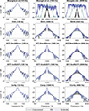 |
Figure 19. Magnitude spectra of unprocessed audiometric signals and corresponding simulator outputs for the mild and moderate degree of hearing loss conditions. The peak value for each condition was normalised to 0 dB to facilitate comparison. Note the wider frequency range depicted on the abscissa for Mourgela, 1000 Hz and 8000 Hz. |
When leaving overall level changes out of consideration, the effect of the magnitude spectra processing appears to be rather subtle for a majority of the simulators. In most cases, only the side lobes of the spectra showed increased levels compared to the reference signal, while the width of the main lobe remained unchanged. In some cases, additional spectral artifacts were present outside of the frequency ranges depicted here, but with levels well below those of the main lobe and side lobes close to it.
A notable exception was the Mourgela simulator: Its smearing method produced distinctly different results from the other simulators. For 125 Hz, the behaviour was similar to that for the other simulators for both the mild and the moderate condition. For 1 kHz and 8 kHz, the behaviour changed and a pronounced spectral broadening in the shape of a noise-like plateau around the centre frequency emerged. The effect was clear for the mild condition and was even more pronounced for the moderate condition (note the wider frequency range depicted on the abscissa). This frequency-dependent difference in results was expected, as the smearing processing is applied only to frequency bands above 729 Hz for this simulator.
Similar to the observations regarding the input-output functions, there were no clear differences between the two frequency smearing methods Baer&Moore and Graf&3DTI of the 3DTI simulator.
4 Discussion and conclusion
In this contribution, four software tools for the simulation of hearing loss were introduced and evaluated. The statistical analyses of the perceptual results provided evidence that the simulators yielded results significantly different from one another when used to simulate elevated hearing thresholds for normal-hearing listeners. It was also shown that the simulation performance and accuracy strongly depended on the degree of the simulated hearing loss and the frequency. When simulating elevated hearing thresholds, the most accurate results were obtained using the WHIS simulator, especially for the moderate degree of hearing loss. For this simulator, only seven out of the 14 tested conditions showed significant deviations from the target value. Median values did not deviate by more than 5 dB from the target hearing threshold levels across the range of tested frequencies. Since commonly used systems for hearing loss classification utilize steps of 15 or 20 dB [50], these results support the applicability of the WHIS simulator – at least for the simulation of elevated hearing thresholds. Deviations of varying degree were observed for the other simulators. Particularly for the frequency of 8 kHz, the measured hearing thresholds were lower than the defined target values for the Mourgela, 3DTI, and Clarity simulators (for both the mild and moderate hearing losses). Note that for this evaluation, the VST-plugin version of the 3DTI simulator was used. Differing results might be observed with the C++ library version, as some differences between values of pre-configured parameters were found when comparing the code of the library and the code of the VST-plugin.
Concerning the precision of results of the listening experiments, the measurement uncertainty according to ISO 8253-1 [45] of the pure-tone audiometry method should be considered, with uncertainty contributions such as uncertainties for repeated measures, audiometric equipment, as well as transducers and their fitting. The procedure for the compilation of uncertainty contributions described in ISO 8253-1 yields the following results for the expanded measurement uncertainty for 95% coverage probability: a value of 10 dB for frequencies up to and including 4 kHz (for measurements with a step size of 3 dB or 5 dB), a value of 14 dB above 4 kHz when testing with a step size of 5 dB (as was used in Experiment 1), and a value of 13 dB above 4 kHz when testing with a step size of 3 dB (as was used in Experiment 2). Thus, even when employing an ideal hearing loss simulator, perfect results cannot be expected. In particular, testing with a step size of, e.g., 5 dB, may result in a small overestimation of the hearing threshold. For example, in a given situation the true hearing threshold of a participant may be between 10 and 15 dB HL; testing with 10 dB HL will likely not elicit a response from the participant. When the next available step, 15 dB HL, is tested, a response will likely be elicited, but the recorded threshold of 15 dB HL is slightly higher than the true threshold.
Regarding the two different experiment environments in which testing took place, no noticeable effect of the rooms on the results was expected or observed. Both the anechoic chamber and the isolated hearing booth feature highly absorptive surfaces and very low ambient noise levels, which meet the requirements defined in ISO 8253-1 [45] for threshold determination in the range of 125 Hz to 8 kHz down to hearing levels of −10 dB HL.
Overall, the input-output functions introduced and discussed in Section 3.1 were well-suited to predict the perceptual results (i.e., the increase in hearing thresholds) and to depict and assess the non-linear nature of the processing involved. While the good suitability of this metric was expected to a certain extent, the conducted listening experiments proved to be an important validation of the method. Together with the discussed measurement uncertainty of the audiometry method used, any observed mismatch between predicted values and corresponding perceptual results may originate from other alterations to the input signal caused by the simulator (which cannot be observed directly when inspecting reduced RMS output hearing levels), such as time-varying behaviour of the expander processing in the context of loudness recruitment simulation.
In comparison to other processing steps involved during the simulation, the spectral smearing, intended to decrease the frequency resolution of the listener’s hearing, proved to be rather subtle in most cases – at least for the sinusoidal signals discussed here; more pronounced effects might be observed for other test signals, e.g., narrow-band noise. A notable exception was the simulator of Mourgela et al., which employs a more pronounced spectral broadening processing. The observation of similar results for the frequency smearing of the Clarity and 3DTI (with setting Baer&Moore) simulators seems reasonable: While using different approaches for other aspects of the simulation, they both employ an implementation of the spectral smearing method of Baer & Moore [17, 18]. Even though the second frequency smearing option of the 3DTI simulator, Graf&3DTI, was developed based on findings by different researchers, the results were highly similar to the ones obtained using the option Baer&Moore.
The required accuracy of a specific simulation will depend on the context of its application. For example, the requirements of a recording engineer interested in getting an approximate impression of how a mix might sound for a person with hearing loss may be less rigorous than for the conduct of listening experiments or assisting the development of hearing aid algorithms.
5 Limitations and outlook
Considering the complexity of the auditory system and its potential disorders, additional studies are needed to assess the hearing loss simulators’ effect on several other auditory properties not covered in the study presented here. These may investigate the extent to which the simulators are able to successfully reproduce existing impairments such as increased auditory filter bandwidth, reduced resolution of temporal-spectral modulation detection, changes in forward masking, poorer speech recognition in noise, and loudness recruitment. Suitable methods for a perceptual evaluation of the latter may include the Short Increment Sensitivity Index (SISI) test [51], the Fowler test [52], and the Adaptive Categorical Loudness Scaling (ACALOS) test [53].
Resolving the problem of deviating audiometric results observed in the case of a majority of the evaluated simulators seems desirable. In general, interesting options and challenges for future developments and advances in the field of hearing loss simulation remain. Along with an increase in realism or accuracy of the simulated aspects covered in this evaluation, these may include the integration of additional aspects, such as the simulation of diplacusis, i.e., interaural pitch difference.
Acknowledgments
Parts of the results presented in this contribution were obtained in the context of the master thesis by Sebastian Hillert, written at IHTA under the supervision of the authors. The authors would like to thank Dr. Michael Stone from the University of Manchester for sending the code for the Cambridge Hearing Loss Simulator, as well as Dr. Lorenzo Picinali from the Imperial College London and Dr. Arcadio Reyes Lecuona from the University of Malaga for providing additional information about the 3DTI Hearing Loss Simulator.
Funding
The authors disclosed receipt of the following financial support for the research, authorship, and/or publication of this article: This work was funded by the Deutsche Forschungsgemeinschaft (DFG, German Research Foundation) [project number 513033051].
Conflicts of interest
The authors declare no conflict of interest.
Data availability statement
Data are available on request from the authors.
References
- World Health Organization: World Report on Hearing. World Health Organization, Geneva, 2021. [Google Scholar]
- S.A. Ausili, B. Backus, M.J.H. Agterberg, A. John van Opstal, M.M. van Wanrooij: Sound localization in real-time vocoded cochlear-implant simulations with normal-hearing listeners. Trends in Hearing 23 (2019) 2331216519847332. [CrossRef] [Google Scholar]
- A.A. Kressner, T. May, T. Dau: Effect of noise reduction gain errors on simulated cochlear implant speech intelligibility. Trends in Hearing 23 (2019) 2331216519825930. [Google Scholar]
- B.C.J. Moore: Perceptual consequences of cochlear hearing loss and their implications for the design of hearing aids. Ear and Hearing 17, 2 (1996) 133–161. [Google Scholar]
- B.C.J. Moore, Cochlear Hearing Loss: Physiological, Psychological and Technical Issues. John Wiley & Sons, 2 edition, 2007. [Google Scholar]
- D. Schwarz, Hearing-Loss Visualizer, 2023. https://urhear.urmc.rochester.edu/webapps/home/session.html?app=HearingLossVisualizer. [Google Scholar]
- N. Grimault, T. Irino, S. Dimachki, A. Corneyllie, R.D. Patterson, S. Garcia: A real time hearing loss simulator. Acta Acustica united with Acustica, 104, 5 (2018) 904–908. [Google Scholar]
- D.S. Lum, L.D. Braida: Perception of speech and non-speech sounds by listeners with real and simulated sensorineural hearing loss. Journal of Phonetics 28, 3 (2000) 343–366. [Google Scholar]
- H. Kayser, T. Herzke, P. Maanen, M. Zimmermann, G. Grimm, V. Hohmann: Open community platform for hearing aid algorithm research: open Master Hearing Aid (openMHA). SoftwareX 17 (2022) 100953. [CrossRef] [PubMed] [Google Scholar]
- T. Herzke: openMHA. https://github.com/HoerTech-gGmbH/openMHA/tree/master/examples/35-hearing-loss-simulation. [Google Scholar]
- J. Grange, M. Zhang, J. Culling: The role of efferent reflexes in the efficient encoding of speech by the auditory nerve. Journal of Neuroscience 42, 36 (2022) 6907–6916. [Google Scholar]
- R. Meddis, W. Lecluyse, N.R. Clark, T. Jürgens, C.M. Tan, M.R. Panda, G.J. Brown: A computer model of the auditory periphery and its application to the study of hearing, in: B.C.J. Moore, R.D. Patterson, I.M. Winter, R.P. Carlyon, H.E. Gockel, Eds. Basic Aspects of Hearing, Vol. 787 of Advances in Experimental Medicine and Biology. Springer New York, New York, NY, 2013, pp. 11–20. [Google Scholar]
- M.J. de Boer, T. Jürgens, F.W. Cornelissen, D. Başkent: Degraded visual and auditory input individually impair audiovisual emotion recognition from speech-like stimuli, but no evidence for an exacerbated effect from combined degradation. Vision Research 180 (2021) 51–62. [Google Scholar]
- T. Jürgens, T. Wesarg, D. Oetting, L. Jung, B. Williges: Spatial speech-in-noise performance in simulated single-sided deaf and bimodal cochlear implant users in comparison with real patients. International Journal of Audiology 62, 1 (2023) 30–43. [Google Scholar]
- The Clarity Team: The Clarity Project, 2024. https://claritychallenge.org/. [Google Scholar]
- Clarity project: ClarityChallenge, 2024. https://github.com/claritychallenge. [Google Scholar]
- T. Baer, B.C.J. Moore: Effects of spectral smearing on the intelligibility of sentences in noise. The Journal of the Acoustical Society of America 94, 3 (1993) 1229–1241. [Google Scholar]
- T. Baer, B.C.J. Moore, Effects of spectral smearing on the intelligibility of sentences in the presence of interfering speech. The Journal of the Acoustical Society of America 95, 4 (1994) 2277–2280. [Google Scholar]
- B.C.J. Moore, B.R. Glasberg: Simulation of the effects of loudness recruitment and threshold elevation on the intelligibility of speech in quiet and in a background of speech. The Journal of the Acoustical Society of America. 94, 4 (1993) 2050–2062. [Google Scholar]
- Y. Nejime, B.C.J. Moore: Simulation of the effect of threshold elevation and loudness recruitment combined with reduced frequency selectivity on the intelligibility of speech in noise. The Journal of the Acoustical Society of America 102, 1 (1997) 603–615. [Google Scholar]
- M.A. Stone, B.C.J. Moore: Tolerable hearing aid delays. I. Estimation of limits imposed by the auditory path alone using simulated hearing losses. Ear and Hearing 20, 3 (1999) 182–192. [CrossRef] [PubMed] [Google Scholar]
- L. Fontan, T. Cretin-Maitenaz, C. Füllgrabe: Predicting speech perception in older listeners with sensorineural hearing loss using automatic speech recognition. Trends in Hearing 24 (2020) 2331216520914769. [Google Scholar]
- ITU-T: Recommendation P.58: Head and torso simulator for telephonometry, 08/1996. [Google Scholar]
- T. Matsui: WHIS: Wadai (or Wakayama University) Hearing Impairment System, 11/2/2020. https://cs.tut.ac.jp/~tmatsui/whis/index-en.html. [Google Scholar]
- T. Irino: WHIS, 2023. https://github.com/AMLAB-Wakayama/WHIS. [Google Scholar]
- T. Irino: Hearing impairment simulator based on auditory excitation pattern playback: WHIS. IEEE Access 11 (2023) 78419–78430. [Google Scholar]
- T. Irino, R.D. Patterson: A time-domain, level-dependent auditory filter: the gammachirp. The Journal of the Acoustical Society of America 101, 1 (1997) 412–419. [Google Scholar]
- T. Irino, R.D. Patterson: A compressive gammachirp auditory filter for both physiological and psychophysical data. The Journal of the Acoustical Society of America 109, 5 Pt 1 (2001) 2008–2022. [Google Scholar]
- T. Irino, R.D. Patterson: A dynamic compressive gammachirp auditory filterbank. IEEE Transactions on Audio, Speech, and Language Processing 14, 6 (2006) 2222–2232. [Google Scholar]
- T. Irino, R.D. Patterson: The gammachirp auditory filter and its application to speech perception. Acoustical Science and Technology 41, 1 (2020) 99–107. [Google Scholar]
- M. Nagae, T. Irino, R. Nisimura, H. Kawahara, R.D. Patterson: Hearing impairment simulator based on compressive gammachirp filter, in: Signal and Information Processing Association Annual Summit and Conference (APSIPA), 2014 Asia-Pacific. IEEE, 2014, pp. 1–4. [Google Scholar]
- R. Meddis: Simulation of mechanical to neural transduction in the auditory receptor. The Journal of the Acoustical Society of America 79, 3 (1986) 702–711. [Google Scholar]
- 3D Tune-In: 3D Tune-In Toolkit, 2023. https://github.com/3DTune-In/3dti_AudioToolkit. [Google Scholar]
- 3D Tune-In: 2015. https://www.3d-tune-in.eu/. [Google Scholar]
- M. Cuevas-Rodríguez, D. González-Toledo, E. La Rubia-Cuestas, C. Garre, L. Molina-Tanco, A. Reyes-Lecuona, D. Poirier-Quinot, L. Picinali: An open-source audio renderer for 3D audio with hearing loss and hearing aid simulations, in: AES Convention 142. Audio Engineering Society, 2017. [Google Scholar]
- M. Cuevas-Rodríguez, D. González-Toledo, E. de La Rubia-Cuestas, C. Garre, L. Molina-Tanco, A. Reyes-Lecuona, D. Poirier-Quinot, L. Picinali: The 3D Tune-In Toolkit – 3D audio spatialiser, hearing loss and hearing aid simulations, in: 2018 IEEE 4th VR Workshop on Sonic Interactions for Virtual Environments (SIVE 2018). IEEE, Piscataway, NJ, 2018, pp. 1–3. [Google Scholar]
- M. Cuevas-Rodríguez, L. Picinali, D. González-Toledo, C. Garre, E. de La Rubia-Cuestas, L. Molina-Tanco, A. Reyes-Lecuona: 3D Tune-In Toolkit: An open-source library for real-time binaural spatialisation. PLoS One 14, 3 (2019) e0211899. [CrossRef] [PubMed] [Google Scholar]
- D.M. Rasetshwane, A.C. Trevino, J.N. Gombert, L. Liebig-Trehearn, J.G. Kopun, W. Jesteadt, S.T. Neely, M.P. Gorga: Categorical loudness scaling and equal-loudness contours in listeners with normal hearing and hearing loss. The Journal of the Acoustical Society of America 137, 4 (2015) 1899–1913. [Google Scholar]
- R. Badri, J.H. Siegel, B.A. Wright: Auditory filter shapes and high-frequency hearing in adults who have impaired speech in noise performance despite clinically normal audiograms. The Journal of the Acoustical Society of America 129, 2 (2011) 852–863. [Google Scholar]
- 3D Tune-In: 3D Tune-In Toolkit features, 2018. https://www.3d-tune-in.eu/sites/default/files/filedepot/3D%20Tune-In%20Toolkit%20Features.pdf. [Google Scholar]
- 3D Tune-In: 3D Tune-In Toolkit Binaural Test Application v4.0 User Manual, 2022. https://github.com/3DTune-In/3dti_AudioToolkit/releases. [Google Scholar]
- A. Mourgela, J. Reiss, T. Agus: Investigation of a real-time hearing loss simulation for use in audio production, in: AES 149th Convention. Audio Engineering Society, 2020. [Google Scholar]
- DIN: Electroacoustics – Audiometric equipment – Part 1: Equipment for pure-tone and speech audiometry, 08/2018. [Google Scholar]
- P. Majdak, C. Hollomey, R. Baumgartner: AMT 1.x: A toolbox for reproducible research in auditory modeling. Acta Acustica 6 (2022) 19. [CrossRef] [EDP Sciences] [Google Scholar]
- ISO: Acoustics – Audiometric test methods – Part 1: Pure-tone air and bone conduction audiometry, 11/01/2010. [Google Scholar]
- ISO: Acoustics – Statistical distribution of hearing thresholds related to age and gender, 01/2017. [Google Scholar]
- M.T. Jacobson and P. Matthews: Generating uniformly distributed random Latin squares. Journal of Combinatorial Designs 4, 6 (1996) 405–437. [Google Scholar]
- P.-Z. Wu, J.T. O’Malley, V. de Gruttola, M. Charles Liberman: Primary neural degeneration in noise-exposed human cochleas: correlations with outer hair cell loss and word-discrimination scores. Journal of Neuroscience 41, 20 (2021) 4439–4447. [Google Scholar]
- JASP Team: JASP, 2024. https://jasp-stats.org/. [Google Scholar]
- J.G. Clark: Uses and abuses of hearing loss classification. ASHA 23, 7 (1981) 493–500. [Google Scholar]
- J. Jerger, J.L. Shedd, E. Harford: On the detection of extremely small changes in sound intensity. A.M.A. Archives of Otolaryngology 69, 2 (1959) 200–211. [Google Scholar]
- E.P. Fowler: The diagnosis of diseases of the neural mechanism of hearing by the aid of sounds well above threshold (presidential address). The Laryngoscope 47, 5 (1937) 289–300. [Google Scholar]
- T. Brand, V. Hohmann: An adaptive procedure for categorical loudness scaling. The Journal of the Acoustical Society of America 112, 4 (2002) 1597–1604. [CrossRef] [PubMed] [Google Scholar]
Appendix A
Experiment 1: Results of one-sample t tests and Bayesian one-sample t tests (Bayes factor BF01 shown in last column).
Experiment 1: Results of repeated measures ANOVA.
Experiment 2: Results of one-sample t tests and Bayesian one-sample t tests (Bayes factor BF01 shown in last column).
Experiment 2: Results of repeated measures ANOVA.
Cite this article as: Deutsch T. Falanga L. Willmes K. Koch I. & Fels J. 2026. Evaluation of elevated hearing thresholds produced by models for the simulation of cochlear hearing loss. Acta Acustica, 10, 14. https://doi.org/10.1051/aacus/2026007.
All Tables
Overview of the hearing loss simulators considered for evaluation in the context of this study, specifying the programming language they are implemented in, whether they are openly available online, whether the signal processing can be achieved in real-time, and whether they can be operated via a graphical user interface (GUI).
Tested audiometric frequencies and corresponding target hearing thresholds (dB HL) for experimental conditions mild and moderate.
Experiment 1: Results of one-sample t tests and Bayesian one-sample t tests (Bayes factor BF01 shown in last column).
Experiment 2: Results of one-sample t tests and Bayesian one-sample t tests (Bayes factor BF01 shown in last column).
All Figures
|
Figure 1. Block diagram depicting the input-output characteristics involved in the simulation of loudness recruitment. |
| In the text | |
|
Figure 2. Block diagram of the processing steps of the Clarity / Cambridge Hearing Loss Simulator. |
| In the text | |
|
Figure 3. Block diagram of the processing steps of the Wadai Hearing Impairment Simulator (WHIS). |
| In the text | |
|
Figure 4. Block diagram of the processing steps of the hearing loss simulator included as part of the 3DTI toolkit. |
| In the text | |
|
Figure 5. Block diagram of the processing steps of the hearing loss simulator of Mourgela et al. |
| In the text | |
|
Figure 6. Implemented temporal envelope of the pulsed tones. Time constants t BC = 21 ms, t EG = 21 ms, t CE = 222 ms, t FJ = 261 ms, t JK = 239 ms meet the requirements defined in DIN EN 60645-1 [43]. |
| In the text | |
|
Figure 7. Auditory spectrogram of the pulsed tone signal with a carrier frequency of 1 kHz. |
| In the text | |
|
Figure 8. Boxplot showing the differences between the hearing thresholds measured using the two audiometry systems. |
| In the text | |
|
Figure 9. Experiment 1: Boxplot showing the hearing threshold results for the mild hearing loss condition. |
| In the text | |
|
Figure 10. Experiment 1: Boxplot showing the hearing threshold results for the moderate hearing loss condition. |
| In the text | |
|
Figure 11. Experiment 1: Mean deviations from the target hearing thresholds for the mild hearing loss condition. Error bars show the 95% CI. |
| In the text | |
|
Figure 12. Experiment 1: Mean deviations from the target hearing thresholds for the moderate hearing loss condition. Error bars show the 95% CI. |
| In the text | |
|
Figure 13. Experiment 2: Boxplot showing the hearing threshold results for the mild hearing loss condition. |
| In the text | |
|
Figure 14. Experiment 2: Boxplot showing the hearing threshold results for the moderate hearing loss condition. |
| In the text | |
|
Figure 15. Experiment 2: Mean deviations from the target hearing thresholds for the mild hearing loss condition. Error bars show the 95% CI. |
| In the text | |
|
Figure 16. Experiment 2: Mean deviations from the target hearing thresholds for the moderate hearing loss condition. Error bars show the 95% CI. |
| In the text | |
|
Figure 17. Input-output functions, i.e., output hearing levels as a function of input hearing level of the audiometric stimuli, for the simulators configured for the mild degree of hearing loss (target hearing thresholds for the different frequencies provided in parentheses). |
| In the text | |
|
Figure 18. Input-output functions, i.e., output hearing levels as a function of input hearing level of the audiometric stimuli, for the simulators configured for the moderate degree of hearing loss (target hearing thresholds for the different frequencies provided in parentheses). |
| In the text | |
|
Figure 19. Magnitude spectra of unprocessed audiometric signals and corresponding simulator outputs for the mild and moderate degree of hearing loss conditions. The peak value for each condition was normalised to 0 dB to facilitate comparison. Note the wider frequency range depicted on the abscissa for Mourgela, 1000 Hz and 8000 Hz. |
| In the text | |
Current usage metrics show cumulative count of Article Views (full-text article views including HTML views, PDF and ePub downloads, according to the available data) and Abstracts Views on Vision4Press platform.
Data correspond to usage on the plateform after 2015. The current usage metrics is available 48-96 hours after online publication and is updated daily on week days.
Initial download of the metrics may take a while.